Posts in category: PyTorch

Recent studies have shown that large model training will be beneficial for improving model quality. During the last 3 years, model size grew 10,000 times from BERT with 110M parameters to Megatron-2 with one trillion. However, training large AI models is not easy—aside from the need for large amounts of computing resources, software engineering complexity is also challenging. PyTorch has been working on building tools and infrastructure to make it easier.

PyTorch Distributed data parallelism is a staple of scalable deep learning because of its robustness and simplicity. It however requires the model to fit on one GPU. Recent approaches like DeepSpeed ZeRO and FairScale’s Fully Sharded Data Parallel allow us to break this barrier by sharding a model’s parameters, gradients and optimizer states across data parallel workers while still maintaining the simplicity of data parallelism.

With PyTorch 1.11 we’re adding native support for Fully Sharded Data Parallel (FSDP), currently available as a prototype feature. Its implementation heavily borrows from FairScale’s version while bringing more streamlined APIs and additional performance improvements.

Scaling tests of PyTorch FSDP on AWS show it can scale up to train dense models with 1T parameters. Realized performance in our experiments reached 84 TFLOPS per A100 GPU for GPT 1T model and 159 TFLOPS per A100 GPU for GPT 175B model on AWS cluster. Native FSDP implementation also dramatically improved model initialization time compared to FairScale’s original when CPU offloading was enabled.

In future PyTorch versions, we’re going to enable users to seamlessly switch between DDP, ZeRO-1, ZeRO-2 and FSDP flavors of data parallelism, so that users can train different scales of models with simple configurations in the unified API.

How FSDP Works

FSDP is a type of data-parallel training, but unlike traditional data-parallel, which maintains a per-GPU copy of a model’s parameters, gradients and optimizer states, it shards all of these states across data-parallel workers and can optionally offload the sharded model parameters to CPUs.

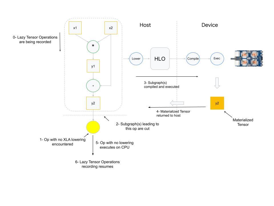
The figure below shows how FSDP works for 2 data-parallel processes:

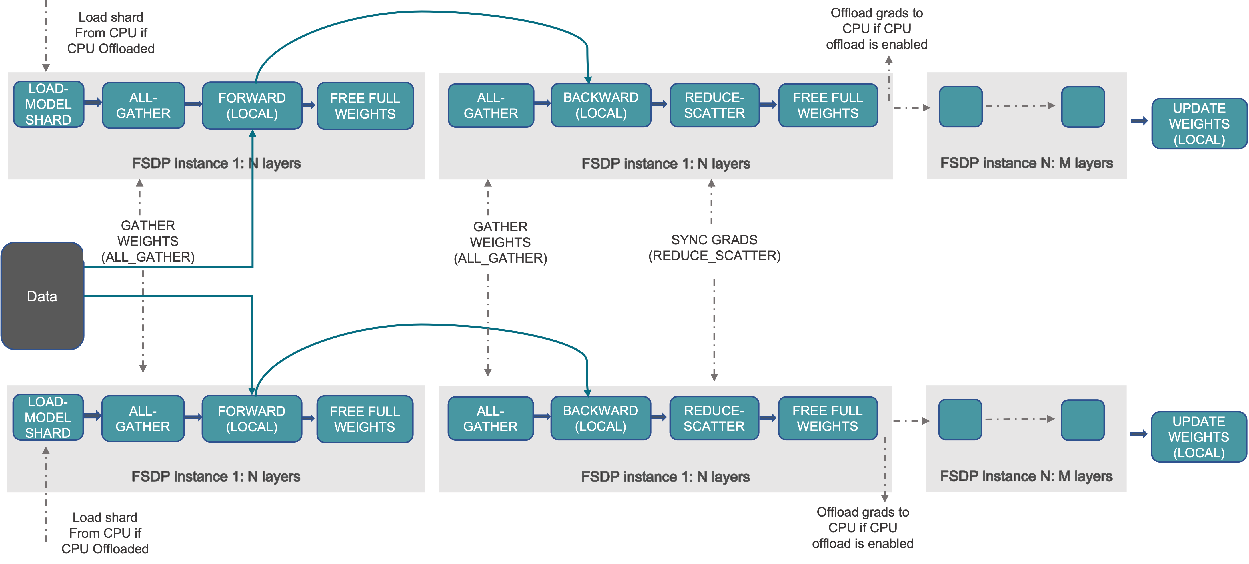
Figure 1. FSDP workflow

Usually, model layers are wrapped with FSDP in a nested way, so that only layers in a single FSDP instance need to gather the full parameters to a single device during forward or backward computations. The gathered full parameters will be freed immediately after computation, and the freed memory can be used for the next layer’s computation. In this way, peak GPU memory could be saved and thus training can be scaled to use a larger model size or larger batch size. To further maximize memory efficiency, FSDP can offload the parameters, gradients and optimizer states to CPUs when the instance is not active in the computation.

Using FSDP in PyTorch

There are two ways to wrap a model with PyTorch FSDP. Auto wrapping is a drop-in replacement for DDP; manual wrapping needs minimal changes of model definition code with the ability to explore complex sharding strategies.

Auto Wrapping

Model layers should be wrapped in FSDP in a nested way to save peak memory and enable communication and computation overlapping. The simplest way to do it is auto wrapping, which can serve as a drop-in replacement for DDP without changing the rest of the code.

fsdp_auto_wrap_policy argument allows specifying a callable function to recursively wrap layers with FSDP. default_auto_wrap_policy function provided by the PyTorch FSDP recursively wraps layers with the number of parameters larger than 100M. You can supply your own wrapping policy as needed. The example of writing a customized wrapping policy is shown in the FSDP API doc.

In addition, cpu_offload could be configured optionally to offload wrapped parameters to CPUs when these parameters are not used in computation. This can further improve memory efficiency at the cost of data transfer overhead between host and device.

The example below shows how FSDP is wrapped using auto wrapping.

from torch.distributed.fsdp import (
   FullyShardedDataParallel,
   CPUOffload,
)
from torch.distributed.fsdp.wrap import (
   default_auto_wrap_policy,
)
import torch.nn as nn
 
class model(nn.Module):
   def __init__(self):
       super().__init__()
       self.layer1 = nn.Linear(8, 4)
       self.layer2 = nn.Linear(4, 16)
       self.layer3 = nn.Linear(16, 4)
 
model = DistributedDataParallel(model())
fsdp_model = FullyShardedDataParallel(
   model(),
   fsdp_auto_wrap_policy=default_auto_wrap_policy,
   cpu_offload=CPUOffload(offload_params=True),
)

Manual Wrapping

Manual wrapping can be useful to explore complex sharding strategies by applying wrap selectively to some parts of the model. Overall settings can be passed to the enable_wrap() context manager.

from torch.distributed.fsdp import (
   FullyShardedDataParallel,
   CPUOffload,
)
from torch.distributed.fsdp.wrap import (
   enable_wrap,
   wrap,
)
import torch.nn as nn
from typing import Dict
 
 
class model(nn.Module):
   def __init__(self):
       super().__init__()
       self.layer1 = wrap(nn.Linear(8, 4))
       self.layer2 = nn.Linear(4, 16)
       self.layer3 = wrap(nn.Linear(16, 4))
 
wrapper_kwargs = Dict(cpu_offload=CPUOffload(offload_params=True))
with enable_wrap(wrapper_cls=FullyShardedDataParallel, **wrapper_kwargs):
   fsdp_model = wrap(model())

After wrapping the model with FSDP using one of the two above approaches, the model can be trained in a similar way as local training, like this:

optim = torch.optim.Adam(fsdp_model.parameters(), lr=0.0001)
for sample, label in next_batch():
  out = fsdp_model(input)
  loss = criterion(out, label)
  loss.backward()
  optim.step()

Benchmark Results

We ran extensive scaling tests for 175B and 1T GPT models on AWS clusters using PyTorch FSDP. Each cluster node is an instance with 8 NVIDIA A100-SXM4-40GB GPUs, and inter-nodes are connected via AWS Elastic Fabric Adapter (EFA) with 400 Gbps network bandwidth.

GPT models are implemented using minGPT. A randomly generated input dataset is used for benchmarking purposes. All experiments ran with 50K vocabulary size, fp16 precision and SGD optimizer.

In addition to using FSDP with parameters CPU offloading in the experiments, the activation checkpointing feature in PyTorch is also applied in the tests.

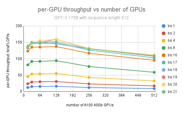
The maximum per-GPU throughput of 159 teraFLOP/s (51% of NVIDIA A100 peak theoretical performance 312 teraFLOP/s/GPU) is achieved with batch size 20 and sequence length 512 on 128 GPUs for the GPT 175B model; further increase of the number of GPUs leads to per-GPU throughput degradation because of growing communication between the nodes.

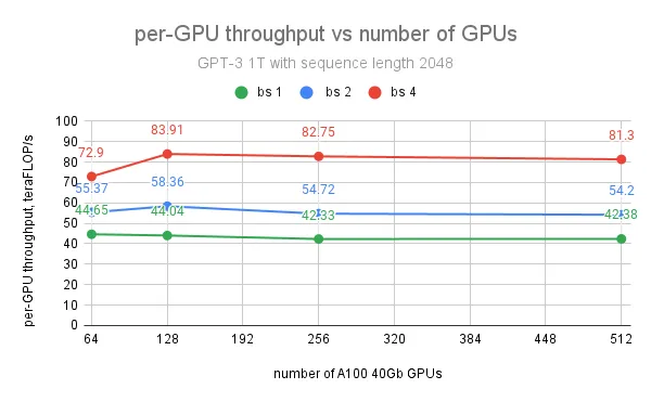
For the GPT 1T model, the maximum per-GPU throughput of 84 teraFLOP/s (27% of the peak teraFLOP/s) is achieved with batch size 4 and sequence length 2048 on 128 GPUs. However, further increase of the number of GPUs doesn’t affect the per-GPU throughput too much because we observed that the largest bottleneck in the 1T model training is not from communication but from the slow CUDA cache allocator when peak GPU memory is reaching the limit. The use of A100 80G GPUs with larger memory capacity will mostly resolve this issue and also help scale the batch size to achieve much larger throughput.

Future Work

In the next beta release, we are planning to add efficient distributed model/states checkpointing APIs, meta device support for large model materialization, and mixed-precision support inside FSDP computation and communication. We’re also going to make it easier to switch between DDP, ZeRO1, ZeRO2 and FSDP flavors of data parallelism in the new API. To further improve FSDP performance, memory fragmentation reduction and communication efficiency improvements are also planned.

A Bit of History of 2 Versions of FSDP

FairScale FSDP was released in early 2021 as part of the FairScale library. And then we started the effort to upstream FairScale FSDP to PyTorch in PT 1.11, making it production-ready. We have selectively upstreamed and refactored key features from FairScale FSDP, redesigned user interfaces and made performance improvements.

In the near future, FairScale FSDP will stay in the FairScale repository for research projects, while generic and widely adopted features will be upstreamed to PyTorch incrementally and hardened accordingly.

Meanwhile, PyTorch FSDP will focus more on production readiness and long-term support. This includes better integration with ecosystems and improvements on performance, usability, reliability, debuggability and composability.

Acknowledgments

We would like to thank the authors of FairScale FSDP: Myle Ott, Sam Shleifer, Min Xu, Priya Goyal, Quentin Duval, Vittorio Caggiano, Tingting Markstrum, Anjali Sridhar. Thanks to the Microsoft DeepSpeed ZeRO team for developing and popularizing sharded data parallel techniques. Thanks to Pavel Belevich, Jessica Choi, Sisil Mehta for running experiments using PyTorch FSDP on different clusters. Thanks to Geeta Chauhan, Mahesh Yadav, Pritam Damania, Dmytro Dzhulgakov for supporting this effort and insightful discussions.

Read More

We are introducing the beta release of TorchRec and a number of improvements to the current PyTorch domain libraries, alongside the PyTorch 1.11 release. These updates demonstrate our focus on developing common and extensible APIs across all domains to make it easier for our community to build ecosystem projects on PyTorch. Highlights include:

• TorchRec, a PyTorch domain library for Recommendation Systems, is available in beta. View it on GitHub.
• TorchAudio – Added Enformer- and RNN-T-based models and recipes to support the full development lifecycle of a streaming ASR model. See the release notes here.
• TorchText – Added beta support for RoBERTa and XLM-R models, byte-level BPE tokenizer, and text datasets backed by TorchData. See the release notes here.
• TorchVision – Added 4 new model families and 14 new classification datasets such as CLEVR, GTSRB, FER2013. See the release notes here.

TorchRec 0.1

We announced TorchRec a few weeks ago and we are excited to release the beta version today. To recap, TorchRec is a PyTorch domain library for Recommendation Systems. This new library provides common sparsity and parallelism primitives, enabling researchers to build state-of-the-art personalization models and deploy them in production. TorchRec was used to train a 1.25 trillion parameter model, pushed to production in January 2022.

In particular, the library includes:

• Modeling primitives, such as embedding bags and jagged tensors, that enable easy authoring of large, performant multi-device/multi-node models using hybrid data-parallelism and model-parallelism.
• Optimized RecSys kernels powered by FBGEMM, including support for sparse and quantized operations.
• A sharder which can partition embedding tables with a variety of different strategies including data-parallel, table-wise, row-wise, table-wise-row-wise, and column-wise sharding.
• A planner which can automatically generate optimized sharding plans for models.
• Pipelining to overlap dataloading device transfer (copy to GPU), inter-device communications (input_dist), and computation (forward, backward) for increased performance.
• GPU inference support.
• Common modules for RecSys, such as models and public datasets (Criteo & Movielens).

Please check the TorchRec announcement post here, video tutorial, install instructions here, test drive the feature through this tutorial here, and refer to the reference document here.

TorchAudio 0.11

TorchAudio: Building Blocks for Audio and Speech Processing

We published a paper, TorchAudio: Building Blocks for Audio and Speech Processing, describing the overview of the TorchAudio library. If you find TorchAudio useful for your research, please help us share with the community by citing our paper.

(Beta) RNN-T & (Prototype) Emformer Models and Recipes

Emformer is an efficient memory-transformer-based streaming acoustic model that has demonstrated state-of-the-art streaming automatic speech recognition (ASR) performance in low-latency, resource-constrained scenarios, such as on-device applications (citation: https://arxiv.org/abs/2010.10759).

The TorchAudio v0.11 release includes the following beta features:

• Implementation of Emformer (docs)
• Recurrent neural network transducer (RNN-T) streaming ASR model that uses Emformer for its transcription network (docs)
• RNN-T beam search decoder with TorchScript support (docs)
• LibriSpeech Emformer RNN-T training recipe (GitHub) and corresponding pre-trained streaming ASR inference pipeline (docs)

Also there are prototype features that are available from nightly builds or the main branch.

• Training recipes trained on MuST-C and TED-LIUM3 datasets. (GitHub)
• Pre-trained pipelines corresponding to the recipes. (docs)
• Tutorial that steps through performing online speech recognition with RNN-T Emformer model. (docs)

Collectively, these features cover the full development lifecycle of a streaming ASR model, from definition through training and inference, and enable users to easily develop their own Emformer- and RNN-T-based models.

Special thanks to Yangyang Shi, Jay Mahadeokar, and Gil Keren for their code contributions and guidance.

(Beta) HuBERT Pretrain Model

The masked prediction training of HuBERT model requires the masked logits, unmasked logits, and feature norm as the outputs. The logits are for cross-entropy losses and the feature norm is for penalty loss. The release adds HuBERTPretrainModel and corresponding factory functions (hubert_pretrain_base, hubert_pretrain_large, and hubert_pretrain_xlarge) to enable training from scratch.

(Prototype) CTC Beam Search Decoder

In recent releases, TorchAudio has added support for ASR models fine-tuned on CTC loss. The addition of an inference time CTC beam search decoder enables running end-to-end ASR evaluation using TorchAudio utils.

The CTC decoder in TorchAudio supports customizable beam search decoding with lexicon constraint. It also has optional KenLM language model support.

For more details, please check out the API tutorial and documentation. This prototype feature is available through nightly builds.

(Prototype) Streaming API

TorchAudio started as simple audio I/O APIs that supplement PyTorch. With the recent addition of ASR models and training recipes, the project has received requests to support high-level application development.

Streaming API makes it easy to develop and test the model in online inference. It utilizes ffmpeg under the hood, and enables reading media from online services and hardware devices, decoding media in an incremental manner, and applying filters and preprocessing.

Please checkout the API tutorial and the documentation. There are also the streaming ASR tutorial and the device streaming ASR tutorial. This feature is available from nightly releases. Please refer to pytorch.org for how to install nightly builds.

TorchText 0.12

(Beta) RoBERTa and XLM-R Models

TorchText has added support for pre-trained RoBERTa and XLM-R models. It would allow users to train end-2-end Transformer Encoder based models on standard NLP tasks using TorchText.

More specifically:

• The models are torchscriptable and hence can be employed for production use-cases.
• The model APIs let users to easily attach custom task-specific heads with pre-trained encoders.
• The API also comes equipped with data pre-processing transforms to match the pre-trained weights and model configuration.

We have added a tutorial to demonstrate SST-2 binary text classification task with pre-trained XLM-R base architecture.

For additional details on model APIs and usage examples, please refer to the documentation.

(Beta) byte-level BPE tokenizer

TorchText has added support for a Byte-Level BPE tokenizer, as used in GPT-2. This tokenizer is also used for tokenizing inputs to the pre-trained RoBERTa models described previously. In addition to the RoBERTa vocab, users can also load their own custom BPE vocab to use the tokenizer. Furthermore, the tokenizer is fully torchscriptable and hence can be employed for production use-cases. For additional details on model APIs and usage examples, please refer to the documentation.

(Beta) Text datasets backed by TorchData

TorchText has modernized its datasets by migrating from older-style Iterable Datasets to TorchData’s DataPipes. TorchData is a library that provides modular/composable primitives, allowing users to load and transform data in performant data pipelines.

These DataPipes work out-of-the-box with PyTorch DataLoader and would enable new functionalities like auto-sharding. Users can now easily do data manipulation and pre-processing using user-defined functions and transformations in a functional style programming. Datasets backed by DataPipes also enable standard flow-control like batching, collation, shuffling and bucketizing.

Collectively, DataPipes provides a comprehensive experience for data preprocessing and tensorization needs in a pythonic and flexible way for model training. We have added a tutorial to demonstrate data-processing pipelining using the modernized dataset for binary text-classification.

You can learn more about TorchData DataPipe APIs in its official documentation.

TorchVision 0.12

New Models

Four new model families have been released in the latest version along with pre-trained weights for their variants.

#1 Object Detection

FCOS is a popular, fully convolutional, anchor-free model for object detection. In this release we include a community-contributed model implementation as well as pre-trained weights. The model was trained on COCO train2017 and can be used as follows:

import torch
from torchvision import models

x = [torch.rand(3, 224, 224)]
fcos = models.detection.fcos_resnet50_fpn(pretrained=True).eval()
predictions =  fcos(x)

The box AP of the pre-trained model on COCO val2017 is 39.2 (see #4961 for more details).

We would like to thank Hu Ye and Zhiqiang Wang for contributing to the model implementation and initial training. This was the first community-contributed model in a long while, and given its success, we decided to use the learnings from this process and create a new model contribution guidelines.

#2 Optical Flow support and RAFT model

TorchVision now supports optical flow! Optical Flow models try to predict movement in a video: given two consecutive frames, the model predicts where each pixel of the first frame ends up in the second frame. Check out our new tutorial on Optical Flow!

We implemented a torchscript-compatible RAFT model with pre-trained weights (both normal and “small” versions), and added support for training and evaluating optical flow models. Our training scripts support distributed training across processes and nodes, leading to much faster training time than the original implementation. We also added 5 new optical flow datasets: Flying Chairs, Flying Things, Sintel, Kitti, and HD1K.

#3. Image Classification

Vision Transformer (ViT) and ConvNeXt are two popular architectures which can be used as image classifiers or as backbones for downstream vision tasks. In this release we include 8 pre-trained weights for their classification variants. The models were trained on ImageNet and can be used as follows:

import torch
from torchvision import models

x = torch.rand(1, 3, 224, 224)
vit = models.detection.vit_b_16(pretrained=True).eval()
convnext = models.detection.convnext_tiny(pretrained=True).eval()
predictions1 = vit(x)
predictions2 = convnext(x)

The accuracies of the pre-trained models obtained on ImageNet val are seen below:

The above models have been trained using an adjusted version of our new training recipe and this allows us to offer models with accuracies significantly higher than the ones on the original papers.

#4. GPU Video Decoding

In this release, we add support for GPU video decoding in the video reading API. To use hardware-accelerated decoding, we just need to pass a cuda device to the video reading API as shown below:

import torchvision

reader = torchvision.io.VideoReader(file_name, device="cuda:0")
for frame in reader:
    print(frame)

We also support seeking to anyframe or a keyframe in the video before reading, as shown below:

reader.seek(seek_time)

New Datasets

We have implemented 14 new classification datasets: CLEVR, GTSRB, FER2013, SUN397, Country211, Flowers102, fvgc_aircraft, OxfordIIITPet, DTD, Food 101, Rendered SST2, Stanford cars, PCAM, and EuroSAT.

As part of our work on Optical Flow support (see above for more details), we also added 5 new optical flow datasets: Flying Chairs, Flying Things, Sintel, Kitti, and HD1K.

Other Updates

• New documentation layout: Each function / class is now documented in a separate page, clearing up some space in the per-module pages, and easing the discovery of the proposed APIs. Compare e.g. our previous docs vs the new ones. Please let us know if you have any feedback!
• New model contribution guidelines have been published following the success of the FCOS model which was contributed by the community. These guidelines aim to be an overview of the model contribution process for anyone who would like to suggest, implement and train a new model.
• Upcoming Prototype API – We are currently working on a prototype API which adds Multi-weight support on all of our model builder methods. This will enable us to offer multiple pre-trained weights, associated with their meta-data and inference transforms. The API is still under review and thus was not included in the release but you can read more about it on our blogpost and provide your feedback on the dedicated Github issue.
• Changes in our deprecation policy – Up until now, torchvision would almost never remove deprecated APIs. In order to be more aligned and consistent with pytorch core, we are updating our deprecation policy. We are now following a 2-release deprecation cycle: deprecated APIs will raise a warning for 2 versions, and will be removed after that. To reflect these changes and to smooth the transition, we have decided to:
  • Remove all APIs that had been deprecated before or on v0.8, released 1.5 years ago.
  • Update the removal timeline of all other deprecated APIs to v0.14, to reflect the new 2-cycle policy starting now in v0.12.

Captum 0.5

Captum is a PyTorch library for model interpretability. For this release, we expanded Captum with influential instances and added support for both similarity based influences and novel algorithms, TracIn and its variants. TracIn variants offer faster approximation of influence scores based on random projections for fully connected layers.

More specifically the new, influence, subsection of Captum includes:

• SimilarityInfluence computes similarity scores between test and training examples using default (cosine or euclidean) or custom user definite metrics w.r.t. given input model layers.
• TracInCP approximates the influential score of each training example on a given test example based on the dot-product similarity between loss gradients w.r.t. model parameters for test and training examples. Note that if we use training examples as test examples then we compute self influence. This method and its variants described below also return top-k proponents and opponents which are the top-k largest positive and negative influential examples respectively.
• TracInCPFast is an approximation of TracInCP that avoids computing the gradients w.r.t. large parameter matrices. It approximates influence score based on the dot products between last fully connected layer activations and loss gradients w.r.t. that layer for training and test examples.
• TracInCPFastRandProj uses a nearest neighbor approximation library such as annoy to compute the dot product between the training and test quantities. In order to reduce the dimensionality of layer activations and corresponding gradients this method, in addition, allows to project those vectors into a lower dimensional space using random projection matrices.

More about the implementation of influential instances can be found on our GitHub page and tutorials.

Thanks for reading, If you’re interested in these updates and want to join the PyTorch community, we encourage you to join the discussion forums and open GitHub issues. To get the latest news from PyTorch, follow us on Twitter, Medium, YouTube, and LinkedIn.

Cheers!

Team PyTorch

Read More

Introduction

Ease of use, expressivity, and debuggability are among the core principles of PyTorch. One of the key drivers for the ease of use is that PyTorch execution is by default “eager, i.e. op by op execution preserves the imperative nature of the program. However, eager execution does not offer the compiler based optimization, for example, the optimizations when the computation can be expressed as a graph.

LazyTensor [1], first introduced with PyTorch/XLA, helps combine these seemingly disparate approaches. While PyTorch eager execution is widely used, intuitive, and well understood, lazy execution is not as prevalent yet.

In this post we will explore some of the basic concepts of the LazyTensor System with the goal of applying these concepts to understand and debug performance of LazyTensor based implementations in PyTorch. Although we will use PyTorch/XLA on Cloud TPU as the vehicle for exploring these concepts, we hope that these ideas will be useful to understand other system(s) built on LazyTensors.

LazyTensor

Any operation performed on a PyTorch tensor is by default dispatched as a kernel or a composition of kernels to the underlying hardware. These kernels are executed asynchronously on the underlying hardware. The program execution is not blocked until the value of a tensor is fetched. This approach scales extremely well with massively parallel programmed hardware such as GPUs.

The starting point of a LazyTensor system is a custom tensor type. In PyTorch/XLA, this type is called XLA tensor. In contrast to PyTorch’s native tensor type, operations performed on XLA tensors are recorded into an IR graph. Let’s examine an example that sums the product of two tensors:

import torch
import torch_xla
import torch_xla.core.xla_model as xm

dev = xm.xla_device()

x1 = torch.rand((3, 3)).to(dev)
x2 = torch.rand((3, 8)).to(dev)

y1 = torch.einsum('bs,st->bt', x1, x2)
print(torch_xla._XLAC._get_xla_tensors_text([y1]))

You can execute this colab notebook to examine the resulting graph for y1. Notice that no computation has been performed yet.

y1 = y1 + x2
print(torch_xla._XLAC._get_xla_tensors_text([y1]))

The operations will continue until PyTorch/XLA encounters a barrier. This barrier can either be a mark step() api call or any other event which forces the execution of the graph recorded so far.

xm.mark_step()
print(torch_xla._XLAC._get_xla_tensors_text([y1]))

Once the mark_step() is called, the graph is compiled and then executed on TPU, i.e. the tensors have been materialized. Therefore, the graph is now reduced to a single line y1 tensor which holds the result of the computation.

Compile Once, Execute Often

XLA compilation passes offer optimizations (e.g. op-fusion, which reduces HBM pressure by using scratch-pad memory for multiple ops, ref ) and leverages lower level XLA infrastructure to optimally use the underlying hardware. However, there is one caveat, compilation passes are expensive, i.e. can add to the training step time. Therefore, this approach scales well if and only if we can compile once and execute often (compilation cache helps, such that the same graph is not compiled more than once).

In the following example, we create a small computation graph and time the execution:

y1 = torch.rand((3, 8)).to(dev)
def dummy_step() :
  y1 = torch.einsum('bs,st->bt', y1, x)
  xm.mark_step()
  return y1

%timeit dummy_step

The slowest run took 29.74 times longer than the fastest. This could mean that an intermediate result is being cached.
10000000 loops, best of 5: 34.2 ns per loop

You notice that the slowest step is quite longer than the fastest. This is because of the graph compilation overhead which is incurred only once for a given shape of graph, input shape, and output shape. Subsequent steps are faster because no graph compilation is necessary.

This also implies that we expect to see performance cliffs when the “compile once and execute often” assumption breaks. Understanding when this assumption breaks is the key to understanding and optimizing the performance of a LazyTensor system. Let’s examine what triggers the compilation.

Graph Compilation and Execution and LazyTensor Barrier

We saw that the computation graph is compiled and executed when a LazyTensor barrier is encountered. There are three scenarios when the LazyTensor barrier is automatically or manually introduced. The first is the explicit call of mark_step() api as shown in the preceding example. mark_step() is also called implicitly at every step when you wrap your dataloader with MpDeviceLoader (highly recommended to overlap compute and data upload to TPU device). The Optimizer step method of xla_model also allows to implicitly call mark_step (when you set barrier=True).

The second scenario where a barrier is introduced is when PyTorch/XLA finds an op with no mapping (lowering) to equivalent XLA HLO ops. PyTorch has 2000+ operations. Although most of these operations are composite (i.e. can be expressed in terms of other fundamental operations), some of these operations do not have corresponding lowering in XLA.

What happens when an op with no XLA lowering is used? PyTorch XLA stops the operation recording and cuts the graph(s) leading to the input(s) of the unlowered op. This cut graph is then compiled and dispatched for execution. The results (materialized tensor) of execution are sent back from device to host, the unlowered op is then executed on the host (cpu), and then downstream LazyTensor operations creating a new graph(s) until a barrier is encountered again.

The third and final scenario which results in a LazyTensor barrier is when there is a control structure/statement or another method which requires the value of a tensor. This statement would at the minimum cause the execution of the computation graph leading to the tensor (if the graph has already been seen) or cause compilation and execution of both.

Other examples of such methods include .item(), isEqual(). In general, any operation that maps Tensor -> Scalar will cause this behavior.

Dynamic Graph

As illustrated in the preceding section, graph compilation cost is amortized if the same shape of the graph is executed many times. It’s because the compiled graph is cached with a hash derived from the graph shape, input shape, and the output shape. If these shapes change it will trigger compilation, and too frequent compilation will result in training time degradation.

Let’s consider the following example:

def dummy_step(x, y, loss, acc=False):
  z = torch.einsum('bs,st->bt', y, x)
  step_loss = z.sum().view(1,)
  if acc:
    loss = torch.cat((loss, step_loss))
  else:
    loss = step_loss
  xm.mark_step()
  return loss


import time
def measure_time(acc=False):
  exec_times = []
  iter_count = 100
  x = torch.rand((512, 8)).to(dev)
  y = torch.rand((512, 512)).to(dev)
  loss = torch.zeros(1).to(dev)
  for i in range(iter_count):
    tic = time.time()
    loss = dummy_step(x, y, loss, acc=acc)
    toc = time.time()
    exec_times.append(toc - tic)
  return exec_times

dyn = measure_time(acc=True) # acc= True Results in dynamic graph
st = measure_time(acc=False) # Static graph, computation shape, inputs and output shapes don't change

import matplotlib.pyplot as plt
plt.plot(st, label = 'static graph')
plt.plot(dyn, label = 'dynamic graph')
plt.legend()
plt.title('Execution time in seconds')

Note that static and dynamic cases have the same computation but dynamic graph compiles every time, leading to the higher overall run-time. In practice, the training step with recompilation can sometimes be an order of magnitude or slower. In the next section we discuss some of the PyTorch/XLA tools to debug training degradation.

Profiling Training Performance with PyTorch/XLA

PyTorch/XLA profiling consists of two major components. First is the client side profiling. This feature is turned on by simply setting the environment variable PT_XLA_DEBUG to 1. Client side profiling points to unlowered ops or device-to-host transfer in your source code. Client side profiling also reports if there are too frequent compilations happening during the training. You can explore some metrics and counters provided by PyTorch/XLA in conjunction with the profiler in this notebook.

The second component offered by PyTorch/XLA profiler is the inline trace annotation. For example:

import torch_xla.debug.profiler as xp

def train_imagenet():
  print('==> Preparing data..')
  img_dim = get_model_property('img_dim')
  ....
  server = xp.start_server(3294)
  def train_loop_fn(loader, epoch):
    ....
    model.train()
    for step, (data, target) in enumerate(loader):
      with xp.StepTrace('Train_Step', step_num=step):
        ....
        if FLAGS.amp:
        ....
        else:
          with xp.Trace('build_graph'):
            output = model(data)
            loss = loss_fn(output, target)
            loss.backward()
          xm.optimizer_step(optimizer)

Notice the start_server api call. The port number that you have used here is the same port number you will use with the tensorboard profiler in order to view the op trace similar to:

Op trace along with the client-side debugging function is a powerful set of tools to debug and optimize your training performance with PyTorch/XLA. For more detailed instructions on the profiler usage, the reader is encouraged to explore blogs part-1, part-2, and part-3 of the blog series on PyTorch/XLA performance debugging.

Summary

In this article we have reviewed the fundamentals of the LazyTensor system. We built on those fundamentals with PyTorch/XLA to understand the potential causes of training performance degradation. We discussed why “compile once and execute often” helps to get the best performance on LazyTensor systems, and why training slows down when this assumption breaks.

We hope that PyTorch users will find these insights helpful for their novel works with LazyTensor systems.

Acknowledgements

A big thank you to my outstanding colleagues Jack Cao, Milad Mohammedi, Karl Weinmeister, Rajesh Thallam, Jordan Tottan (Google) and Geeta Chauhan (Meta) for their meticulous reviews and feedback. And thanks to the extended PyTorch/XLA development team from Google, Meta, and the open source community to make PyTorch possible on TPUs. And finally, thanks to the authors of the LazyTensor paper not only for developing LazyTensor but also for writing such an accessible paper.

Refrences

Read More

Amazon Ads uses PyTorch, TorchServe, and AWS Inferentia to reduce inference costs by 71% and drive scale out.

Amazon Ads helps companies build their brand and connect with shoppers through ads shown both within and beyond Amazon’s store, including websites, apps, and streaming TV content in more than 15 countries. Businesses and brands of all sizes, including registered sellers, vendors, book vendors, Kindle Direct Publishing (KDP) authors, app developers, and agencies can upload their own ad creatives, which can include images, video, audio, and, of course, products sold on Amazon.

To promote an accurate, safe, and pleasant shopping experience, these ads must comply with content guidelines. For example, ads cannot flash on and off, products must be featured in an appropriate context, and images and text should be appropriate for a general audience. To help ensure that ads meet the required policies and standards, we needed to develop scalable mechanisms and tools.

As a solution, we used machine learning (ML) models to surface ads that might need revision. As deep neural networks flourished over the past decade, our data science team began exploring more versatile deep learning (DL) methods capable of processing text, images, audio, or video with minimal human intervention. To that end, we’ve used PyTorch to build computer vision (CV) and natural language processing (NLP) models that automatically flag potentially non-compliant ads. PyTorch is intuitive, flexible, and user-friendly, and has made our transition to using DL models seamless. Deploying these new models on AWS Inferentia-based Amazon EC2 Inf1 instances, rather than on GPU-based instances, reduced our inference latency by 30 percent and our inference costs by 71 percent for the same workloads.

Transition to deep learning

Our ML systems paired classical models with word embeddings to evaluate ad text. But our requirements evolved, and as the volume of submissions continued to expand, we needed a method nimble enough to scale along with our business. In addition, our models must be fast and serve ads within milliseconds to provide an optimal customer experience.

Over the last decade, DL has become very popular in numerous domains, including natural language, vision, and audio. Because deep neural networks channel data sets through many layers — extracting progressively higher-level features — they can make more nuanced inferences than classical ML models. Rather than simply detecting prohibited language, for example, a DL model can reject an ad for making false claims.

In addition, DL techniques are transferable– a model trained for one task can be adapted to carry out a related task. For instance, a pre-trained neural network can be optimized to detect objects in images and then fine-tuned to identify specific objects that are not allowed to be displayed in an ad.

Deep neural networks can automate two of classical ML’s most time-consuming steps: feature engineering and data labeling. Unlike traditional supervised learning approaches, which require exploratory data analysis and hand-engineered features, deep neural networks learn the relevant features directly from the data. DL models can also analyze unstructured data, like text and images, without the preprocessing necessary in ML. Deep neural networks scale effectively with more data and perform especially well in applications involving large data sets.

We chose PyTorch to develop our models because it helped us maximize the performance of our systems. With PyTorch, we can serve our customers better while taking advantage of Python’s most intuitive concepts. The programming in PyTorch is object-oriented: it groups processing functions with the data they modify. As a result, our codebase is modular, and we can reuse pieces of code in different applications. In addition, PyTorch’s eager mode allows loops and control structures and, therefore, more complex operations in the model. Eager mode makes it easy to prototype and iterate upon our models, and we can work with various data structures. This flexibility helps us update our models quickly to meet changing business requirements.

“Before this, we experimented with other frameworks that were “Pythonic,” but PyTorch was the clear winner for us here.” said Yashal Kanungo, Applied Scientist. “Using PyTorch was easy because the structure felt native to Python programming, which the data scientists were very familiar with”.

Training pipeline

Today, we build our text models entirely in PyTorch. To save time and money, we often skip the early stages of training by fine-tuning a pre-trained NLP model for language analysis. If we need a new model to evaluate images or video, we start by browsing PyTorch’s torchvision library, which offers pretrained options for image and video classification, object detection, instance segmentation, and pose estimation. For specialized tasks, we build a custom model from the ground up. PyTorch is perfect for this, because eager mode and the user-friendly front end make it easy to experiment with different architectures.

To learn how to finetune neural networks in PyTorch, head to this tutorial.

Before we begin training, we optimize our model’s hyperparameters, the variables that define the network architecture (for example, the number of hidden layers) and training mechanics (such as learning rate and batch size). Choosing appropriate hyperparameter values is essential, because they will shape the training behavior of the model. We rely on the Bayesian search feature in SageMaker, AWS’s ML platform, for this step. Bayesian search treats hyperparameter tuning as a regression problem: It proposes the hyperparameter combinations that are likely to produce the best results and runs training jobs to test those values. After each trial, a regression algorithm determines the next set of hyperparameter values to test, and performance improves incrementally.

We prototype and iterate upon our models using SageMaker Notebooks. Eager mode lets us prototype models quickly by building a new computational graph for each training batch; the sequence of operations can change from iteration to iteration to accommodate different data structures or to jibe with intermediate results. That frees us to adjust the network during training without starting over from scratch. These dynamic graphs are particularly valuable for recursive computations based on variable sequence lengths, such as the words, sentences, and paragraphs in an ad that are analyzed with NLP.

When we’ve finalized the model architecture, we deploy training jobs on SageMaker. PyTorch helps us develop large models faster by running numerous training jobs at the same time. PyTorch’s Distributed Data Parallel (DDP) module replicates a single model across multiple interconnected machines within SageMaker, and all the processes run forward passes simultaneously on their own unique portion of the data set. During the backward pass, the module averages the gradients of all the processes, so each local model is updated with the same parameter values.

Model deployment pipeline

When we deploy the model in production, we want to ensure lower inference costs without impacting prediction accuracy. Several PyTorch features and AWS services have helped us address the challenge.

The flexibility of a dynamic graph enriches training, but in deployment we want to maximize performance and portability. An advantage of developing NLP models in PyTorch is that out of the box, they can be traced into a static sequence of operations by TorchScript, a subset of Python specialized for ML applications. Torchscript converts PyTorch models to a more efficient, production-friendly intermediate representation (IR) graph that is easily compiled. We run a sample input through the model, and TorchScript records the operations executed during the forward pass. The resulting IR graph can run in high-performance environments, including C++ and other multithreaded Python-free contexts, and optimizations such as operator fusion can speed up the runtime.

Neuron SDK and AWS Inferentia powered compute

We deploy our models on Amazon EC2 Inf1 instances powered by AWS Inferentia, Amazon’s first ML silicon designed to accelerate deep learning inference workloads. Inferentia has shown to reduce inference costs by up to 70% compared to Amazon EC2 GPU-based instances.
We used the AWS Neuron SDK — a set of software tools used with Inferentia — to compile and optimize our models for deployment on EC2 Inf1 instances.

The code snippet below shows how to compile a Hugging Face BERT model with Neuron. Like torch.jit.trace(), neuron.trace() records the model’s operations on an example input during the forward pass to build a static IR graph.

import torch
from transformers import BertModel, BertTokenizer
import torch.neuron
tokenizer = BertTokenizer.from_pretrained("path to saved vocab")
model = BertModel.from_pretrained("path to the saved model", returned_dict=False)
inputs = tokenizer ("sample input", return_tensor="pt")
neuron_model = torch.neuron.trace(model,
                                  example_inputs = (inputs['input_ids'], inputs['attention_mask']),
                                  verbose = 1)
output = neuron_model(*(inputs['input_ids'], inputs['attention_mask']))

Autocasting and recalibration

Under the hood, Neuron optimizes our models for performance by autocasting them to a smaller data type. As a default, most applications represent neural network values in the 32-bit single-precision floating point (FP32) number format. Autocasting the model to a 16-bit format — half-precision floating point (FP16) or Brain Floating Point (BF16) — reduces a model’s memory footprint and execution time. In our case, we decided to use FP16 to optimize for performance while maintaining high accuracy.

Autocasting to a smaller data type can, in some cases, trigger slight differences in the model’s predictions. To ensure that the model’s accuracy is not affected, Neuron compares the performance metrics and predictions of the FP16 and FP32 models. When autocasting diminishes the model’s accuracy, we can tell the Neuron compiler to convert only the weights and certain data inputs to FP16, keeping the rest of the intermediate results in FP32. In addition, we often run a few iterations with the training data to recalibrate our autocasted models. This process is much less intensive than the original training.

Deployment

To analyze multimedia ads, we run an ensemble of DL models. All ads uploaded to Amazon are run through specialized models that assess every type of content they include: images, video and audio, headlines, texts, backgrounds, and even syntax, grammar, and potentially inappropriate language. The signals we receive from these models indicate whether or not an advertisement complies with our criteria.

Deploying and monitoring multiple models is significantly complex, so we depend on TorchServe, SageMaker’s default PyTorch model serving library. Jointly developed by Facebook’s PyTorch team and AWS to streamline the transition from prototyping to production, TorchServe helps us deploy trained PyTorch models at scale without having to write custom code. It provides a secure set of REST APIs for inference, management, metrics, and explanations. With features such as multi-model serving, model versioning, ensemble support, and automatic batching, TorchServe is ideal for supporting our immense workload. You can read more about deploying your Pytorch models on SageMaker with native TorchServe integration in this blog post.

In some use cases, we take advantage of PyTorch’s object-oriented programming paradigm to wrap multiple DL models into one parent object — a PyTorch nn.Module — and serve them as a single ensemble. In other cases, we use TorchServe to serve individual models on separate SageMaker endpoints, running on AWS Inf1 instances.

Custom handlers

We particularly appreciate that TorchServe allows us to embed our model initialization, preprocessing, inferencing, and post processing code in a single Python script, handler.py, which lives on the server. This script — the handler —preprocesses the un-labeled data from an ad, runs that data through our models, and delivers the resulting inferences to downstream systems. TorchServe provides several default handlers that load weights and architecture and prepare the model to run on a particular device. We can bundle all the additional required artifacts, such as vocabulary files or label maps, with the model in a single archive file.

When we need to deploy models that have complex initialization processes or that originated in third-party libraries, we design custom handlers in TorchServe. These let us load any model, from any library, with any required process. The following snippet shows a simple handler that can serve Hugging Face BERT models on any SageMaker hosting endpoint instance.

import torch
import torch.neuron
from ts.torch_handler.base_handler import BaseHandler
import transformers
from transformers import AutoModelForSequenceClassification,AutoTokenizer

class MyModelHandler(BaseHandler):
    def initialize(self, context):
        self.manifest = ctx.manifest
        properties = ctx.system_properties
        model_dir = properties.get("model_dir")
        serialized_file = self.manifest["model"]["serializedFile"]
        model_pt_path = os.path.join(model_dir, serialized_file)


        self.tokenizer = AutoTokenizer.from_pretrained(
                model_dir, do_lower_case=True
            )
        self.model = AutoModelForSequenceClassification.from_pretrained(
                    model_dir
                )

    def preprocess(self, data):

        input_text = data.get("data")
        if input_text is None:
            input_text = data.get("body")
            inputs = self.tokenizer.encode_plus(input_text, max_length=int(max_length), pad_to_max_length=True, add_special_tokens=True, return_tensors='pt')
        return inputs

    def inference(self,inputs):
        predictions = self.model(**inputs)
        return predictions

    def postprocess(self, output):
        return output

Batching

Hardware accelerators are optimized for parallelism, and batching — feeding a model multiple inputs in a single step — helps saturate all available capacity, typically resulting in higher throughputs. Excessively high batch sizes, however, can increase latency with minimal improvement in throughputs. Experimenting with different batch sizes helps us identify the sweet spot for our models and hardware accelerator. We run experiments to determine the best batch size for our model size, payload size, and request traffic patterns.

The Neuron compiler now supports variable batch sizes. Previously, tracing a model hardcoded the predefined batch size, so we had to pad our data, which can waste compute, slow throughputs, and exacerbate latency. Inferentia is optimized to maximize throughput for small batches, reducing latency by easing the load on the system.

Parallelism

Model parallelism on multi-cores also improves throughput and latency, which is crucial for our heavy workloads. Each Inferentia chip contains four NeuronCores that can either run separate models simultaneously or form a pipeline to stream a single model. In our use case, the data parallel configuration offers the highest throughput at the lowest cost, because it scales out concurrent processing requests.

Data Parallel:

Model Parallel:

Monitoring

It is critical that we monitor the accuracy of our inferences in production. Models that initially make good predictions can eventually degrade in deployment as they are exposed to a wider variety of data. This phenomenon, called model drift, usually occurs when the input data distributions or the prediction targets change.

We use SageMaker Model Monitor to track parity between the training and production data. Model Monitor notifies us when predictions in production begin to deviate from the training and validation results. Thanks to this early warning, we can restore accuracy — by retraining the model if necessary — before our advertisers are affected. To track performance in real time, Model Monitor also sends us metrics about the quality of predictions, such as accuracy, F-scores, and the distribution of the predicted classes.

To determine if our application needs to scale, TorchServe logs resource utilization metrics for the CPU, Memory, and Disk at regular intervals; it also records the number of requests received versus the number served. For custom metrics, TorchServe offers a Metrics API.

A rewarding result

Our DL models, developed in PyTorch and deployed on Inferentia, sped up our ads analysis while cutting costs. Starting with our first explorations in DL, programming in PyTorch felt natural. Its user-friendly features helped smooth the course from our early experiments to the deployment of our multimodal ensembles. PyTorch lets us prototype and build models quickly, which is vital as our advertising service evolves and expands. For an added benefit, PyTorch works seamlessly with Inferentia and our AWS ML stack. We look forward to building more use cases with PyTorch, so we can continue to serve our clients accurate, real-time results.

Read More

We are excited to announce TorchRec, a PyTorch domain library for Recommendation Systems. This new library provides common sparsity and parallelism primitives, enabling researchers to build state-of-the-art personalization models and deploy them in production.

How did we get here?

Recommendation Systems (RecSys) comprise a large footprint of production-deployed AI today, but you might not know it from looking at Github. Unlike areas like Vision and NLP, much of the ongoing innovation and development in RecSys is behind closed company doors. For academic researchers studying these techniques or companies building personalized user experiences, the field is far from democratized. Further, RecSys as an area is largely defined by learning models over sparse and/or sequential events, which has large overlaps with other areas of AI. Many of the techniques are transferable, particularly for scaling and distributed execution. A large portion of the global investment in AI is in developing these RecSys techniques, so cordoning them off blocks this investment from flowing into the broader AI field.

By mid-2020, the PyTorch team received a lot of feedback that there hasn’t been a large-scale production-quality recommender systems package in the open-source PyTorch ecosystem. While we were trying to find a good answer, a group of engineers at Meta wanted to contribute Meta’s production RecSys stack as a PyTorch domain library, with a strong commitment to growing an ecosystem around it. This seemed like a good idea that benefits researchers and companies across the RecSys domain. So, starting from Meta’s stack, we began modularizing and designing a fully-scalable codebase that is adaptable for diverse recommendation use-cases. Our goal was to extract the key building blocks from across Meta’s software stack to simultaneously enable creative exploration and scale. After nearly two years, a battery of benchmarks, migrations, and testing across Meta, we’re excited to finally embark on this journey together with the RecSys community. We want this package to open a dialogue and collaboration across the RecSys industry, starting with Meta as the first sizable contributor.

Introducing TorchRec

TorchRec includes a scalable low-level modeling foundation alongside rich batteries-included modules. We initially target “two-tower” ([1], [2]) architectures that have separate submodules to learn representations of candidate items and the query or context. Input signals can be a mix of floating point “dense” features or high-cardinality categorical “sparse” features that require large embedding tables to be trained. Efficient training of such architectures involves combining data parallelism that replicates the “dense” part of computation and model parallelism that partitions large embedding tables across many nodes.

In particular, the library includes:

• Modeling primitives, such as embedding bags and jagged tensors, that enable easy authoring of large, performant multi-device/multi-node models using hybrid data-parallelism and model-parallelism.
• Optimized RecSys kernels powered by FBGEMM , including support for sparse and quantized operations.
• A sharder which can partition embedding tables with a variety of different strategies including data-parallel, table-wise, row-wise, table-wise-row-wise, and column-wise sharding.
• A planner which can automatically generate optimized sharding plans for models.
• Pipelining to overlap dataloading device transfer (copy to GPU), inter-device communications (input_dist), and computation (forward, backward) for increased performance.
• GPU inference support.
• Common modules for RecSys, such as models and public datasets (Criteo & Movielens).

To showcase the flexibility of this tooling, let’s look at the following code snippet, pulled from our DLRM Event Prediction example:

# Specify the sparse embedding layers
eb_configs = [
   EmbeddingBagConfig(
       name=f"t_{feature_name}",
       embedding_dim=64,
       num_embeddings=100_000,
       feature_names=[feature_name],
   )
   for feature_idx, feature_name in enumerate(DEFAULT_CAT_NAMES)
]

# Import and instantiate the model with the embedding configuration
# The "meta" device indicates lazy instantiation, with no memory allocated
train_model = DLRM(
   embedding_bag_collection=EmbeddingBagCollection(
       tables=eb_configs, device=torch.device("meta")
   ),
   dense_in_features=len(DEFAULT_INT_NAMES),
   dense_arch_layer_sizes=[512, 256, 64],
   over_arch_layer_sizes=[512, 512, 256, 1],
   dense_device=device,
)

# Distribute the model over many devices, just as one would with DDP.
model = DistributedModelParallel(
   module=train_model,
   device=device,
)

optimizer = torch.optim.SGD(params, lr=args.learning_rate)
# Optimize the model in a standard loop just as you would any other model!
# Or, you can use the pipeliner to synchronize communication and compute
for epoch in range(epochs):
   # Train

Scaling Performance

TorchRec has state-of-the-art infrastructure for scaled Recommendations AI, powering some of the largest models at Meta. It was used to train a 1.25 trillion parameter model, pushed to production in January, and a 3 trillion parameter model which will be in production soon. This should be a good indication that PyTorch is fully capable of the largest scale RecSys problems in industry. We’ve heard from many in the community that sharded embeddings are a pain point. TorchRec cleanly addresses that. Unfortunately it is challenging to provide large-scale benchmarks with public datasets, as most open-source benchmarks are too small to show performance at scale.

Looking ahead

Open-source and open-technology have universal benefits. Meta is seeding the PyTorch community with a state-of-the-art RecSys package, with the hope that many join in on building it forward, enabling new research and helping many companies. The team behind TorchRec plan to continue this program indefinitely, building up TorchRec to meet the needs of the RecSys community, to welcome new contributors, and to continue to power personalization at Meta. We’re excited to begin this journey and look forward to contributions, ideas, and feedback!

References

Read More

Quantization is a cheap and easy way to make your DNN run faster and with lower memory requirements. PyTorch offers a few different approaches to quantize your model. In this blog post, we’ll lay a (quick) foundation of quantization in deep learning, and then take a look at how each technique looks like in practice. Finally we’ll end with recommendations from the literature for using quantization in your workflows.

Fig 1. PyTorch <3 Quantization

Contents

• Fundamentals of Quantization
  • Mapping function
  • Quantization Parameters
  • Calibration
  • Affine and Symmetric Quantization Schemes
  • Per-Tensor and Per-Channel Quantization Schemes
  • Backend Engine
  • QConfig
• In PyTorch
  • Post-Training Dynamic/Weight-only Quantization
  • Post-Training Static Quantization (PTQ)
  • Quantization-aware Training (QAT)
• Sensitivity Analysis
• Recommendations for your workflow
  • Points to note
• References

Fundamentals of Quantization

If someone asks you what time it is, you don’t respond “10:14:34:430705”, but you might say “a quarter past 10”.

Quantization has roots in information compression; in deep networks it refers to reducing the numerical precision of its weights and/or activations.

Overparameterized DNNs have more degrees of freedom and this makes them good candidates for information compression [1]. When you quantize a model, two things generally happen – the model gets smaller and runs with better efficiency. Hardware vendors explicitly allow for faster processing of 8-bit data (than 32-bit data) resulting in higher throughput. A smaller model has lower memory footprint and power consumption [2], crucial for deployment at the edge.

Mapping function

The mapping function is what you might guess – a function that maps values from floating-point to integer space. A commonly used mapping function is a linear transformation given by , where is the input and are quantization parameters.

To reconvert to floating point space, the inverse function is given by .

, and their difference constitutes the quantization error.

Quantization Parameters

The mapping function is parameterized by the scaling factor and zero-point .

is simply the ratio of the input range to the output range

where [] is the clipping range of the input, i.e. the boundaries of permissible inputs. [] is the range in quantized output space that it is mapped to. For 8-bit quantization, the output range .

acts as a bias to ensure that a 0 in the input space maps perfectly to a 0 in the quantized space.

Calibration

The process of choosing the input clipping range is known as calibration. The simplest technique (also the default in PyTorch) is to record the running mininmum and maximum values and assign them to and . TensorRT also uses entropy minimization (KL divergence), mean-square-error minimization, or percentiles of the input range.

In PyTorch, Observer modules (docs, code) collect statistics on the input values and calculate the qparams . Different calibration schemes result in different quantized outputs, and it’s best to empirically verify which scheme works best for your application and architecture (more on that later).

from torch.quantization.observer import MinMaxObserver, MovingAverageMinMaxObserver, HistogramObserver
C, L = 3, 4
normal = torch.distributions.normal.Normal(0,1)
inputs = [normal.sample((C, L)), normal.sample((C, L))]
print(inputs)

# >>>>>
# [tensor([[-0.0590,  1.1674,  0.7119, -1.1270],
#          [-1.3974,  0.5077, -0.5601,  0.0683],
#          [-0.0929,  0.9473,  0.7159, -0.4574]]]),

# tensor([[-0.0236, -0.7599,  1.0290,  0.8914],
#          [-1.1727, -1.2556, -0.2271,  0.9568],
#          [-0.2500,  1.4579,  1.4707,  0.4043]])]

observers = [MinMaxObserver(), MovingAverageMinMaxObserver(), HistogramObserver()]
for obs in observers:
  for x in inputs: obs(x) 
  print(obs.__class__.__name__, obs.calculate_qparams())

# >>>>>
# MinMaxObserver (tensor([0.0112]), tensor([124], dtype=torch.int32))
# MovingAverageMinMaxObserver (tensor([0.0101]), tensor([139], dtype=torch.int32))
# HistogramObserver (tensor([0.0100]), tensor([106], dtype=torch.int32))

Affine and Symmetric Quantization Schemes

Affine or asymmetric quantization schemes assign the input range to the min and max observed values. Affine schemes generally offer tighter clipping ranges and are useful for quantizing non-negative activations (you don’t need the input range to contain negative values if your input tensors are never negative). The range is calculated as
. Affine quantization leads to more computationally expensive inference when used for weight tensors [3].

Symmetric quantization schemes center the input range around 0, eliminating the need to calculate a zero-point offset. The range is calculated as
. For skewed signals (like non-negative activations) this can result in bad quantization resolution because the clipping range includes values that never show up in the input (see the pyplot below).

act =  torch.distributions.pareto.Pareto(1, 10).sample((1,1024))
weights = torch.distributions.normal.Normal(0, 0.12).sample((3, 64, 7, 7)).flatten()

def get_symmetric_range(x):
  beta = torch.max(x.max(), x.min().abs())
  return -beta.item(), beta.item()

def get_affine_range(x):
  return x.min().item(), x.max().item()

def plot(plt, data, scheme):
  boundaries = get_affine_range(data) if scheme == 'affine' else get_symmetric_range(data)
  a, _, _ = plt.hist(data, density=True, bins=100)
  ymin, ymax = np.quantile(a[a>0], [0.25, 0.95])
  plt.vlines(x=boundaries, ls='--', colors='purple', ymin=ymin, ymax=ymax)

fig, axs = plt.subplots(2,2)
plot(axs[0, 0], act, 'affine')
axs[0, 0].set_title("Activation, Affine-Quantized")

plot(axs[0, 1], act, 'symmetric')
axs[0, 1].set_title("Activation, Symmetric-Quantized")

plot(axs[1, 0], weights, 'affine')
axs[1, 0].set_title("Weights, Affine-Quantized")

plot(axs[1, 1], weights, 'symmetric')
axs[1, 1].set_title("Weights, Symmetric-Quantized")
plt.show()

Fig 2. Clipping ranges (in purple) for affine and symmetric schemes

In PyTorch, you can specify affine or symmetric schemes while initializing the Observer. Note that not all observers support both schemes.

for qscheme in [torch.per_tensor_affine, torch.per_tensor_symmetric]:
  obs = MovingAverageMinMaxObserver(qscheme=qscheme)
  for x in inputs: obs(x)
  print(f"Qscheme: {qscheme} | {obs.calculate_qparams()}")

# >>>>>
# Qscheme: torch.per_tensor_affine | (tensor([0.0101]), tensor([139], dtype=torch.int32))
# Qscheme: torch.per_tensor_symmetric | (tensor([0.0109]), tensor([128]))

Per-Tensor and Per-Channel Quantization Schemes

Quantization parameters can be calculated for the layer’s entire weight tensor as a whole, or separately for each channel. In per-tensor, the same clipping range is applied to all the channels in a layer

Fig 3. Per-Channel uses one set of qparams for each channel. Per-tensor uses the same qparams for the entire tensor.

For weights quantization, symmetric-per-channel quantization provides better accuracies; per-tensor quantization performs poorly, possibly due to high variance in conv weights across channels from batchnorm folding [3].

from torch.quantization.observer import MovingAveragePerChannelMinMaxObserver
obs = MovingAveragePerChannelMinMaxObserver(ch_axis=0)  # calculate qparams for all `C` channels separately
for x in inputs: obs(x)
print(obs.calculate_qparams())

# >>>>>
# (tensor([0.0090, 0.0075, 0.0055]), tensor([125, 187,  82], dtype=torch.int32))

Backend Engine

Currently, quantized operators run on x86 machines via the FBGEMM backend, or use QNNPACK primitives on ARM machines. Backend support for server GPUs (via TensorRT and cuDNN) is coming soon. Learn more about extending quantization to custom backends: RFC-0019.

backend = 'fbgemm' if x86 else 'qnnpack'
qconfig = torch.quantization.get_default_qconfig(backend)  
torch.backends.quantized.engine = backend

QConfig

The QConfig (code, docs) NamedTuple stores the Observers and the quantization schemes used to quantize activations and weights.

Be sure to pass the Observer class (not the instance), or a callable that can return Observer instances. Use with_args() to override the default arguments.

my_qconfig = torch.quantization.QConfig(
  activation=MovingAverageMinMaxObserver.with_args(qscheme=torch.per_tensor_affine),
  weight=MovingAveragePerChannelMinMaxObserver.with_args(qscheme=torch.qint8)
)
# >>>>>
# QConfig(activation=functools.partial(<class 'torch.ao.quantization.observer.MovingAverageMinMaxObserver'>, qscheme=torch.per_tensor_affine){}, weight=functools.partial(<class 'torch.ao.quantization.observer.MovingAveragePerChannelMinMaxObserver'>, qscheme=torch.qint8){})

In PyTorch

PyTorch allows you a few different ways to quantize your model depending on

• if you prefer a flexible but manual, or a restricted automagic process (Eager Mode v/s FX Graph Mode)
• if qparams for quantizing activations (layer outputs) are precomputed for all inputs, or calculated afresh with each input (static v/s dynamic),
• if qparams are computed with or without retraining (quantization-aware training v/s post-training quantization)

FX Graph Mode automatically fuses eligible modules, inserts Quant/DeQuant stubs, calibrates the model and returns a quantized module – all in two method calls – but only for networks that are symbolic traceable. The examples below contain the calls using Eager Mode and FX Graph Mode for comparison.

In DNNs, eligible candidates for quantization are the FP32 weights (layer parameters) and activations (layer outputs). Quantizing weights reduces the model size. Quantized activations typically result in faster inference.

As an example, the 50-layer ResNet network has ~26 million weight parameters and computes ~16 million activations in the forward pass.

Post-Training Dynamic/Weight-only Quantization

Here the model’s weights are pre-quantized; the activations are quantized on-the-fly (“dynamic”) during inference. The simplest of all approaches, it has a one line API call in torch.quantization.quantize_dynamic. Currently only Linear and Recurrent (LSTM, GRU, RNN) layers are supported for dynamic quantization.

(+) Can result in higher accuracies since the clipping range is exactly calibrated for each input [1].

(+) Dynamic quantization is preferred for models like LSTMs and Transformers where writing/retrieving the model’s weights from memory dominate bandwidths [4].

(-) Calibrating and quantizing the activations at each layer during runtime can add to the compute overhead.

import torch
from torch import nn

# toy model
m = nn.Sequential(
  nn.Conv2d(2, 64, (8,)),
  nn.ReLU(),
  nn.Linear(16,10),
  nn.LSTM(10, 10))

m.eval()

## EAGER MODE
from torch.quantization import quantize_dynamic
model_quantized = quantize_dynamic(
    model=m, qconfig_spec={nn.LSTM, nn.Linear}, dtype=torch.qint8, inplace=False
)

## FX MODE
from torch.quantization import quantize_fx
qconfig_dict = {"": torch.quantization.default_dynamic_qconfig}  # An empty key denotes the default applied to all modules
model_prepared = quantize_fx.prepare_fx(m, qconfig_dict)
model_quantized = quantize_fx.convert_fx(model_prepared)

Post-Training Static Quantization (PTQ)

PTQ also pre-quantizes model weights but instead of calibrating activations on-the-fly, the clipping range is pre-calibrated and fixed (“static”) using validation data. Activations stay in quantized precision between operations during inference. About 100 mini-batches of representative data are sufficient to calibrate the observers [2]. The examples below use random data in calibration for convenience – using that in your application will result in bad qparams.

Fig 4. Steps in Post-Training Static Quantization

Module fusion combines multiple sequential modules (eg: [Conv2d, BatchNorm, ReLU]) into one. Fusing modules means the compiler needs to only run one kernel instead of many; this speeds things up and improves accuracy by reducing quantization error.

(+) Static quantization has faster inference than dynamic quantization because it eliminates the float<->int conversion costs between layers.

(-) Static quantized models may need regular re-calibration to stay robust against distribution-drift.

# Static quantization of a model consists of the following steps:

#     Fuse modules
#     Insert Quant/DeQuant Stubs
#     Prepare the fused module (insert observers before and after layers)
#     Calibrate the prepared module (pass it representative data)
#     Convert the calibrated module (replace with quantized version)

import torch
from torch import nn

backend = "fbgemm"  # running on a x86 CPU. Use "qnnpack" if running on ARM.

m = nn.Sequential(
     nn.Conv2d(2,64,3),
     nn.ReLU(),
     nn.Conv2d(64, 128, 3),
     nn.ReLU()
)

## EAGER MODE
"""Fuse
- Inplace fusion replaces the first module in the sequence with the fused module, and the rest with identity modules
"""
torch.quantization.fuse_modules(m, ['0','1'], inplace=True) # fuse first Conv-ReLU pair
torch.quantization.fuse_modules(m, ['2','3'], inplace=True) # fuse second Conv-ReLU pair

"""Insert stubs"""
m = nn.Sequential(torch.quantization.QuantStub(), 
                  *m, 
                  torch.quantization.DeQuantStub())

"""Prepare"""
m.qconfig = torch.quantization.get_default_qconfig(backend)
torch.quantization.prepare(m, inplace=True)

"""Calibrate
- This example uses random data for convenience. Use representative (validation) data instead.
"""
with torch.inference_mode():
  for _ in range(10):
    x = torch.rand(1,2, 28, 28)
    m(x)
    
"""Convert"""
torch.quantization.convert(m, inplace=True)

"""Check"""
print(m[[1]].weight().element_size()) # 1 byte instead of 4 bytes for FP32


## FX GRAPH
from torch.quantization import quantize_fx
m.eval()
qconfig_dict = {"": torch.quantization.get_default_qconfig(backend)}
# Prepare
model_prepared = quantize_fx.prepare_fx(model_to_quantize, qconfig_dict)
# Calibrate - Use representative (validation) data.
with torch.inference_mode():
  for _ in range(10):
    x = torch.rand(1,2,28, 28)
    model_prepared(x)
# quantize
model_quantized = quantize_fx.convert_fx(model_prepared)

Quantization-aware Training (QAT)

Fig 5. Steps in Quantization-Aware Training

The PTQ approach is great for large models, but accuracy suffers in smaller models [[6]]. This is of course due to the loss in numerical precision when adapting a model from FP32 to the INT8 realm (Figure 6(a)). QAT tackles this by including this quantization error in the training loss, thereby training an INT8-first model.

Fig 6. Comparison of PTQ and QAT convergence [3]

All weights and biases are stored in FP32, and backpropagation happens as usual. However in the forward pass, quantization is internally simulated via FakeQuantize modules. They are called fake because they quantize and immediately dequantize the data, adding quantization noise similar to what might be encountered during quantized inference. The final loss thus accounts for any expected quantization errors. Optimizing on this allows the model to identify a wider region in the loss function (Figure 6(b)), and identify FP32 parameters such that quantizing them to INT8 does not significantly affect accuracy.

Fig 7. Fake Quantization in the forward and backward pass

Image source: https://developer.nvidia.com/blog/achieving-fp32-accuracy-for-int8-inference-using-quantization-aware-training-with-tensorrt

(+) QAT yields higher accuracies than PTQ.

(+) Qparams can be learned during model training for more fine-grained accuracy (see LearnableFakeQuantize)

(-) Computational cost of retraining a model in QAT can be several hundred epochs [1]

# QAT follows the same steps as PTQ, with the exception of the training loop before you actually convert the model to its quantized version

import torch
from torch import nn

backend = "fbgemm"  # running on a x86 CPU. Use "qnnpack" if running on ARM.

m = nn.Sequential(
     nn.Conv2d(2,64,8),
     nn.ReLU(),
     nn.Conv2d(64, 128, 8),
     nn.ReLU()
)

"""Fuse"""
torch.quantization.fuse_modules(m, ['0','1'], inplace=True) # fuse first Conv-ReLU pair
torch.quantization.fuse_modules(m, ['2','3'], inplace=True) # fuse second Conv-ReLU pair

"""Insert stubs"""
m = nn.Sequential(torch.quantization.QuantStub(), 
                  *m, 
                  torch.quantization.DeQuantStub())

"""Prepare"""
m.train()
m.qconfig = torch.quantization.get_default_qconfig(backend)
torch.quantization.prepare_qat(m, inplace=True)

"""Training Loop"""
n_epochs = 10
opt = torch.optim.SGD(m.parameters(), lr=0.1)
loss_fn = lambda out, tgt: torch.pow(tgt-out, 2).mean()
for epoch in range(n_epochs):
  x = torch.rand(10,2,24,24)
  out = m(x)
  loss = loss_fn(out, torch.rand_like(out))
  opt.zero_grad()
  loss.backward()
  opt.step()

"""Convert"""
m.eval()
torch.quantization.convert(m, inplace=True)

Sensitivity Analysis

Not all layers respond to quantization equally, some are more sensitive to precision drops than others. Identifying the optimal combination of layers that minimizes accuracy drop is time-consuming, so [3] suggest a one-at-a-time sensitivity analysis to identify which layers are most sensitive, and retaining FP32 precision on those. In their experiments, skipping just 2 conv layers (out of a total 28 in MobileNet v1) give them near-FP32 accuracy. Using FX Graph Mode, we can create custom qconfigs to do this easily:

# ONE-AT-A-TIME SENSITIVITY ANALYSIS 

for quantized_layer, _ in model.named_modules():
  print("Only quantizing layer: ", quantized_layer)

  # The module_name key allows module-specific qconfigs. 
  qconfig_dict = {"": None, 
  "module_name":[(quantized_layer, torch.quantization.get_default_qconfig(backend))]}

  model_prepared = quantize_fx.prepare_fx(model, qconfig_dict)
  # calibrate
  model_quantized = quantize_fx.convert_fx(model_prepared)
  # evaluate(model)

Another approach is to compare statistics of the FP32 and INT8 layers; commonly used metrics for these are SQNR (Signal to Quantized Noise Ratio) and Mean-Squre-Error. Such a comparative analysis may also help in guiding further optimizations.

Fig 8. Comparing model weights and activations

PyTorch provides tools to help with this analysis under the Numeric Suite. Learn more about using Numeric Suite from the full tutorial.

# extract from https://pytorch.org/tutorials/prototype/numeric_suite_tutorial.html
import torch.quantization._numeric_suite as ns

def SQNR(x, y):
    # Higher is better
    Ps = torch.norm(x)
    Pn = torch.norm(x-y)
    return 20*torch.log10(Ps/Pn)

wt_compare_dict = ns.compare_weights(fp32_model.state_dict(), int8_model.state_dict())
for key in wt_compare_dict:
    print(key, compute_error(wt_compare_dict[key]['float'], wt_compare_dict[key]['quantized'].dequantize()))

act_compare_dict = ns.compare_model_outputs(fp32_model, int8_model, input_data)
for key in act_compare_dict:
    print(key, compute_error(act_compare_dict[key]['float'][0], act_compare_dict[key]['quantized'][0].dequantize()))

Recommendations for your workflow

Fig 9. Suggested quantization workflow

Click for larger image

Points to note

• Large (10M+ parameters) models are more robust to quantization error. [2]
• Quantizing a model from a FP32 checkpoint provides better accuracy than training an INT8 model from scratch.[2]
• Profiling the model runtime is optional but it can help identify layers that bottleneck inference.
• Dynamic Quantization is an easy first step, especially if your model has many Linear or Recurrent layers.
• Use symmetric-per-channel quantization with MinMax observers for quantizing weights. Use affine-per-tensor quantization with MovingAverageMinMax observers for quantizing activations[2, 3]
• Use metrics like SQNR to identify which layers are most suscpetible to quantization error. Turn off quantization on these layers.
• Use QAT to fine-tune for around 10% of the original training schedule with an annealing learning rate schedule starting at 1% of the initial training learning rate. [3]
• If the above workflow didn’t work for you, we want to know more. Post a thread with details of your code (model architecture, accuracy metric, techniques tried). Feel free to cc me @suraj.pt.

That was a lot to digest, congratulations for sticking with it! Next, we’ll take a look at quantizing a “real-world” model that uses dynamic control structures (if-else, loops). These elements disallow symbolic tracing a model, which makes it a bit tricky to directly quantize the model out of the box. In the next post of this series, we’ll get our hands dirty on a model that is chock full of loops and if-else blocks, and even uses third-party libraries in the forward call.

We’ll also cover a cool new feature in PyTorch Quantization called Define-by-Run, that tries to ease this constraint by needing only subsets of the model’s computational graph to be free of dynamic flow. Check out the Define-by-Run poster at PTDD’21 for a preview.

Thanks to Mark Saroufim for useful comments and feedback!

References

Read More

TorchVision has a new backwards compatible API for building models with multi-weight support. The new API allows loading different pre-trained weights on the same model variant, keeps track of vital meta-data such as the classification labels and includes the preprocessing transforms necessary for using the models. In this blog post, we plan to review the prototype API, show-case its features and highlight key differences with the existing one.

We are hoping to get your thoughts about the API prior finalizing it. To collect your feedback, we have created a Github issue where you can post your thoughts, questions and comments.

Limitations of the current API

TorchVision currently provides pre-trained models which could be a starting point for transfer learning or used as-is in Computer Vision applications. The typical way to instantiate a pre-trained model and make a prediction is:

import torch

from PIL import Image
from torchvision import models as M
from torchvision.transforms import transforms as T


img = Image.open("test/assets/encode_jpeg/grace_hopper_517x606.jpg")

# Step 1: Initialize model
model = M.resnet50(pretrained=True)
model.eval()

# Step 2: Define and initialize the inference transforms
preprocess = T.Compose([
    T.Resize([256, ]),
    T.CenterCrop(224),
    T.PILToTensor(),
    T.ConvertImageDtype(torch.float),
    T.Normalize([0.485, 0.456, 0.406], [0.229, 0.224, 0.225])
])

# Step 3: Apply inference preprocessing transforms
batch = preprocess(img).unsqueeze(0)
prediction = model(batch).squeeze(0).softmax(0)

# Step 4: Use the model and print the predicted category
class_id = prediction.argmax().item()
score = prediction[class_id].item()
with open("imagenet_classes.txt", "r") as f:
    categories = [s.strip() for s in f.readlines()]
    category_name = categories[class_id]
print(f"{category_name}: **** {100 * score}%")

There are a few limitations with the above approach:

1. Inability to support multiple pre-trained weights: Since the pretrained variable is boolean, we can only offer one set of weights. This poses a severe limitation when we significantly improve the accuracy of existing models and we want to make those improvements available to the community. It also stops us from offering pre-trained weights of the same model variant on different datasets.
2. Missing inference/preprocessing transforms: The user is forced to define the necessary transforms prior using the model. The inference transforms are usually linked to the training process and dataset used to estimate the weights. Any minor discrepancies in these transforms (such as interpolation value, resize/crop sizes etc) can lead to major reductions in accuracy or unusable models.
3. Lack of meta-data: Critical pieces of information in relation to the weights are unavailable to the users. For example, one needs to look into external sources and the documentation to find things like the category labels, the training recipe, the accuracy metrics etc.

The new API addresses the above limitations and reduces the amount of boilerplate code needed for standard tasks.

Overview of the prototype API

Let’s see how we can achieve exactly the same results as above using the new API:

from PIL import Image
from torchvision.prototype import models as PM


img = Image.open("test/assets/encode_jpeg/grace_hopper_517x606.jpg")

# Step 1: Initialize model
weights = PM.ResNet50_Weights.ImageNet1K_V1
model = PM.resnet50(weights=weights)
model.eval()

# Step 2: Initialize the inference transforms
preprocess = weights.transforms()

# Step 3: Apply inference preprocessing transforms
batch = preprocess(img).unsqueeze(0)
prediction = model(batch).squeeze(0).softmax(0)

# Step 4: Use the model and print the predicted category
class_id = prediction.argmax().item()
score = prediction[class_id].item()
category_name = weights.meta["categories"][class_id]
print(f"{category_name}: **** {100 * score}**%**")

As we can see the new API eliminates the aforementioned limitations. Let’s explore the new features in detail.

Multi-weight support

At the heart of the new API, we have the ability to define multiple different weights for the same model variant. Each model building method (eg resnet50) has an associated Enum class (eg ResNet50_Weights) which has as many entries as the number of pre-trained weights available. Additionally, each Enum class has a default alias which points to the best available weights for the specific model. This allows the users who want to always use the best available weights to do so without modifying their code.

Here is an example of initializing models with different weights:

from torchvision.prototype.models import resnet50, ResNet50_Weights

# Legacy weights with accuracy 76.130%
model = resnet50(weights=ResNet50_Weights.ImageNet1K_V1)

# New weights with accuracy 80.674%
model = resnet50(weights=ResNet50_Weights.ImageNet1K_V2)

# Best available weights (currently alias for ImageNet1K_V2)
model = resnet50(weights=ResNet50_Weights.default)

# No weights - random initialization
model = resnet50(weights=None)

Associated meta-data & preprocessing transforms

The weights of each model are associated with meta-data. The type of information we store depends on the task of the model (Classification, Detection, Segmentation etc). Typical information includes a link to the training recipe, the interpolation mode, information such as the categories and validation metrics. These values are programmatically accessible via the meta attribute:

from torchvision.prototype.models import ResNet50_Weights

# Accessing a single record
size = ResNet50_Weights.ImageNet1K_V2.meta["size"]

# Iterating the items of the meta-data dictionary
for k, v in ResNet50_Weights.ImageNet1K_V2.meta.items():
    print(k, v)

Additionally, each weights entry is associated with the necessary preprocessing transforms. All current preprocessing transforms are JIT-scriptable and can be accessed via the transforms attribute. Prior using them with the data, the transforms need to be initialized/constructed. This lazy initialization scheme is done to ensure the solution is memory efficient. The input of the transforms can be either a PIL.Image or a Tensor read using torchvision.io.

from torchvision.prototype.models import ResNet50_Weights

# Initializing preprocessing at standard 224x224 resolution
preprocess = ResNet50_Weights.ImageNet1K.transforms()

# Initializing preprocessing at 400x400 resolution
preprocess = ResNet50_Weights.ImageNet1K.transforms(crop_size=400, resize_size=400)

# Once initialized the callable can accept the image data:
# img_preprocessed = preprocess(img)

Associating the weights with their meta-data and preprocessing will boost transparency, improve reproducibility and make it easier to document how a set of weights was produced.

Get weights by name

The ability to link directly the weights with their properties (meta data, preprocessing callables etc) is the reason why our implementation uses Enums instead of Strings. Nevertheless for cases when only the name of the weights is available, we offer a method capable of linking Weight names to their Enums:

from torchvision.prototype.models import get_weight

# Weights can be retrieved by name:
assert get_weight("ResNet50_Weights.ImageNet1K_V1") == ResNet50_Weights.ImageNet1K_V1
assert get_weight("ResNet50_Weights.ImageNet1K_V2") == ResNet50_Weights.ImageNet1K_V2

# Including using the default alias:
assert get_weight("ResNet50_Weights.default") == ResNet50_Weights.ImageNet1K_V2

Deprecations

In the new API the boolean pretrained and pretrained_backbone parameters, which were previously used to load weights to the full model or to its backbone, are deprecated. The current implementation is fully backwards compatible as it seamlessly maps the old parameters to the new ones. Using the old parameters to the new builders emits the following deprecation warnings:

>>> model = torchvision.prototype.models.resnet50(pretrained=True)
 UserWarning: The parameter 'pretrained' is deprecated, please use 'weights' instead.
UserWarning: 
Arguments other than a weight enum or `None` for 'weights' are deprecated. 
The current behavior is equivalent to passing `weights=ResNet50_Weights.ImageNet1K_V1`. 
You can also use `weights=ResNet50_Weights.default` to get the most up-to-date weights.

Additionally the builder methods require using keyword parameters. The use of positional parameter is deprecated and using them emits the following warning:

>>> model = torchvision.prototype.models.resnet50(None)
UserWarning: 
Using 'weights' as positional parameter(s) is deprecated. 
Please use keyword parameter(s) instead.

Testing the new API

Migrating to the new API is very straightforward. The following method calls between the 2 APIs are all equivalent:

# Using pretrained weights:
torchvision.prototype.models.resnet50(weights=ResNet50_Weights.ImageNet1K_V1)
torchvision.models.resnet50(pretrained=True)
torchvision.models.resnet50(True)

# Using no weights:
torchvision.prototype.models.resnet50(weights=None)
torchvision.models.resnet50(pretrained=False)
torchvision.models.resnet50(False)

Note that the prototype features are available only on the nightly versions of TorchVision, so to use it you need to install it as follows:

conda install torchvision -c pytorch-nightly

For alternative ways to install the nightly have a look on the PyTorch download page. You can also install TorchVision from source from the latest main; for more information have a look on our repo.

Accessing state-of-the-art model weights with the new API

If you are still unconvinced about giving a try to the new API, here is one more reason to do so. We’ve recently refreshed our training recipe and achieved SOTA accuracy from many of our models. The improved weights can easily be accessed via the new API. Here is a quick overview of the model improvements:
[Image: chart.png] |Model |Old Acc@1 |New Acc@1 |
|— |— |— |
|EfficientNet B1 |78.642 |79.838 |
|MobileNetV3 Large |74.042 |75.274 |
|Quantized ResNet50 |75.92 |80.282 |
|Quantized ResNeXt101 32x8d |78.986 |82.574 |
|RegNet X 400mf * |72.834 |74.864 |
|RegNet X 800mf * |75.212 |77.522 |
|RegNet X 1 6gf * |77.04 |79.668 |
|RegNet X 3 2gf * |78.364 |81.198 |
|RegNet X 8gf * |79.344 |81.682 |
|RegNet X 16gf * |80.058 |82.72 |
|RegNet X 32gf * |80.622 |83.018 |
|RegNet Y 400mf * |74.046 |75.806 |
|RegNet Y 800mf * |76.42 |78.838 |
|RegNet Y 1 6gf * |77.95 |80.882 |
|RegNet Y 3 2gf * |78.948 |81.984 |
|RegNet Y 8gf * |80.032 |82.828 |
|RegNet Y 16gf * |80.424 |82.89 |
|RegNet Y 32gf * |80.878 |83.366 |
|ResNet50 |76.13 |80.674 |
|ResNet101 |77.374 |81.886 |
|ResNet152 |78.312 |82.284 |
|ResNeXt50 32x4d |77.618 |81.198 |
|ResNeXt101 32x8d |79.312 |82.834 |
|Wide ResNet50 2 |78.468 |81.602 |
|Wide ResNet101 2 |78.848 |82.51 |

• At the time of writing, the RegNet refresh work is in progress, see PR 5107.

Please spare a few minutes to provide your feedback on the new API, as this is crucial for graduating it from prototype and including it in the next release. You can do this on the dedicated Github Issue. We are looking forward to reading your comments!

Read More

TorchVision has a new backwards compatible API for building models with multi-weight support. The new API allows loading different pre-trained weights on the same model variant, keeps track of vital meta-data such as the classification labels and includes the preprocessing transforms necessary for using the models. In this blog post, we plan to review the prototype API, show-case its features and highlight key differences with the existing one.

We are hoping to get your thoughts about the API prior finalizing it. To collect your feedback, we have created a Github issue where you can post your thoughts, questions and comments.

Limitations of the current API

TorchVision currently provides pre-trained models which could be a starting point for transfer learning or used as-is in Computer Vision applications. The typical way to instantiate a pre-trained model and make a prediction is:

import torch

from PIL import Image
from torchvision import models as M
from torchvision.transforms import transforms as T


img = Image.open("test/assets/encode_jpeg/grace_hopper_517x606.jpg")

# Step 1: Initialize model
model = M.resnet50(pretrained=True)
model.eval()

# Step 2: Define and initialize the inference transforms
preprocess = T.Compose([
    T.Resize([256, ]),
    T.CenterCrop(224),
    T.PILToTensor(),
    T.ConvertImageDtype(torch.float),
    T.Normalize([0.485, 0.456, 0.406], [0.229, 0.224, 0.225])
])

# Step 3: Apply inference preprocessing transforms
batch = preprocess(img).unsqueeze(0)
prediction = model(batch).squeeze(0).softmax(0)

# Step 4: Use the model and print the predicted category
class_id = prediction.argmax().item()
score = prediction[class_id].item()
with open("imagenet_classes.txt", "r") as f:
    categories = [s.strip() for s in f.readlines()]
    category_name = categories[class_id]
print(f"{category_name}: **** {100 * score}%")

There are a few limitations with the above approach:

1. Inability to support multiple pre-trained weights: Since the pretrained variable is boolean, we can only offer one set of weights. This poses a severe limitation when we significantly improve the accuracy of existing models and we want to make those improvements available to the community. It also stops us from offering pre-trained weights of the same model variant on different datasets.
2. Missing inference/preprocessing transforms: The user is forced to define the necessary transforms prior using the model. The inference transforms are usually linked to the training process and dataset used to estimate the weights. Any minor discrepancies in these transforms (such as interpolation value, resize/crop sizes etc) can lead to major reductions in accuracy or unusable models.
3. Lack of meta-data: Critical pieces of information in relation to the weights are unavailable to the users. For example, one needs to look into external sources and the documentation to find things like the category labels, the training recipe, the accuracy metrics etc.

The new API addresses the above limitations and reduces the amount of boilerplate code needed for standard tasks.

Overview of the prototype API

Let’s see how we can achieve exactly the same results as above using the new API:

from PIL import Image
from torchvision.prototype import models as PM


img = Image.open("test/assets/encode_jpeg/grace_hopper_517x606.jpg")

# Step 1: Initialize model
weights = PM.ResNet50_Weights.ImageNet1K_V1
model = PM.resnet50(weights=weights)
model.eval()

# Step 2: Initialize the inference transforms
preprocess = weights.transforms()

# Step 3: Apply inference preprocessing transforms
batch = preprocess(img).unsqueeze(0)
prediction = model(batch).squeeze(0).softmax(0)

# Step 4: Use the model and print the predicted category
class_id = prediction.argmax().item()
score = prediction[class_id].item()
category_name = weights.meta["categories"][class_id]
print(f"{category_name}: **** {100 * score}**%**")

As we can see the new API eliminates the aforementioned limitations. Let’s explore the new features in detail.

Multi-weight support

At the heart of the new API, we have the ability to define multiple different weights for the same model variant. Each model building method (eg resnet50) has an associated Enum class (eg ResNet50_Weights) which has as many entries as the number of pre-trained weights available. Additionally, each Enum class has a default alias which points to the best available weights for the specific model. This allows the users who want to always use the best available weights to do so without modifying their code.

Here is an example of initializing models with different weights:

from torchvision.prototype.models import resnet50, ResNet50_Weights

# Legacy weights with accuracy 76.130%
model = resnet50(weights=ResNet50_Weights.ImageNet1K_V1)

# New weights with accuracy 80.674%
model = resnet50(weights=ResNet50_Weights.ImageNet1K_V2)

# Best available weights (currently alias for ImageNet1K_V2)
model = resnet50(weights=ResNet50_Weights.default)

# No weights - random initialization
model = resnet50(weights=None)

Associated meta-data & preprocessing transforms

The weights of each model are associated with meta-data. The type of information we store depends on the task of the model (Classification, Detection, Segmentation etc). Typical information includes a link to the training recipe, the interpolation mode, information such as the categories and validation metrics. These values are programmatically accessible via the meta attribute:

from torchvision.prototype.models import ResNet50_Weights

# Accessing a single record
size = ResNet50_Weights.ImageNet1K_V2.meta["size"]

# Iterating the items of the meta-data dictionary
for k, v in ResNet50_Weights.ImageNet1K_V2.meta.items():
    print(k, v)

Additionally, each weights entry is associated with the necessary preprocessing transforms. All current preprocessing transforms are JIT-scriptable and can be accessed via the transforms attribute. Prior using them with the data, the transforms need to be initialized/constructed. This lazy initialization scheme is done to ensure the solution is memory efficient. The input of the transforms can be either a PIL.Image or a Tensor read using torchvision.io.

from torchvision.prototype.models import ResNet50_Weights

# Initializing preprocessing at standard 224x224 resolution
preprocess = ResNet50_Weights.ImageNet1K.transforms()

# Initializing preprocessing at 400x400 resolution
preprocess = ResNet50_Weights.ImageNet1K.transforms(crop_size=400, resize_size=400)

# Once initialized the callable can accept the image data:
# img_preprocessed = preprocess(img)

Associating the weights with their meta-data and preprocessing will boost transparency, improve reproducibility and make it easier to document how a set of weights was produced.

Get weights by name

The ability to link directly the weights with their properties (meta data, preprocessing callables etc) is the reason why our implementation uses Enums instead of Strings. Nevertheless for cases when only the name of the weights is available, we offer a method capable of linking Weight names to their Enums:

from torchvision.prototype.models import get_weight

# Weights can be retrieved by name:
assert get_weight("ResNet50_Weights.ImageNet1K_V1") == ResNet50_Weights.ImageNet1K_V1
assert get_weight("ResNet50_Weights.ImageNet1K_V2") == ResNet50_Weights.ImageNet1K_V2

# Including using the default alias:
assert get_weight("ResNet50_Weights.default") == ResNet50_Weights.ImageNet1K_V2

Deprecations

In the new API the boolean pretrained and pretrained_backbone parameters, which were previously used to load weights to the full model or to its backbone, are deprecated. The current implementation is fully backwards compatible as it seamlessly maps the old parameters to the new ones. Using the old parameters to the new builders emits the following deprecation warnings:

>>> model = torchvision.prototype.models.resnet50(pretrained=True)
 UserWarning: The parameter 'pretrained' is deprecated, please use 'weights' instead.
UserWarning: 
Arguments other than a weight enum or `None` for 'weights' are deprecated. 
The current behavior is equivalent to passing `weights=ResNet50_Weights.ImageNet1K_V1`. 
You can also use `weights=ResNet50_Weights.default` to get the most up-to-date weights.

Additionally the builder methods require using keyword parameters. The use of positional parameter is deprecated and using them emits the following warning:

>>> model = torchvision.prototype.models.resnet50(None)
UserWarning: 
Using 'weights' as positional parameter(s) is deprecated. 
Please use keyword parameter(s) instead.

Testing the new API

Migrating to the new API is very straightforward. The following method calls between the 2 APIs are all equivalent:

# Using pretrained weights:
torchvision.prototype.models.resnet50(weights=ResNet50_Weights.ImageNet1K_V1)
torchvision.models.resnet50(pretrained=True)
torchvision.models.resnet50(True)

# Using no weights:
torchvision.prototype.models.resnet50(weights=None)
torchvision.models.resnet50(pretrained=False)
torchvision.models.resnet50(False)

Note that the prototype features are available only on the nightly versions of TorchVision, so to use it you need to install it as follows:

conda install torchvision -c pytorch-nightly

For alternative ways to install the nightly have a look on the PyTorch download page. You can also install TorchVision from source from the latest main; for more information have a look on our repo.

Accessing state-of-the-art model weights with the new API

If you are still unconvinced about giving a try to the new API, here is one more reason to do so. We’ve recently refreshed our training recipe and achieved SOTA accuracy from many of our models. The improved weights can easily be accessed via the new API. Here is a quick overview of the model improvements:
[Image: chart.png] |Model |Old Acc@1 |New Acc@1 |
|— |— |— |
|EfficientNet B1 |78.642 |79.838 |
|MobileNetV3 Large |74.042 |75.274 |
|Quantized ResNet50 |75.92 |80.282 |
|Quantized ResNeXt101 32x8d |78.986 |82.574 |
|RegNet X 400mf * |72.834 |74.864 |
|RegNet X 800mf * |75.212 |77.522 |
|RegNet X 1 6gf * |77.04 |79.668 |
|RegNet X 3 2gf * |78.364 |81.198 |
|RegNet X 8gf * |79.344 |81.682 |
|RegNet X 16gf * |80.058 |82.72 |
|RegNet X 32gf * |80.622 |83.018 |
|RegNet Y 400mf * |74.046 |75.806 |
|RegNet Y 800mf * |76.42 |78.838 |
|RegNet Y 1 6gf * |77.95 |80.882 |
|RegNet Y 3 2gf * |78.948 |81.984 |
|RegNet Y 8gf * |80.032 |82.828 |
|RegNet Y 16gf * |80.424 |82.89 |
|RegNet Y 32gf * |80.878 |83.366 |
|ResNet50 |76.13 |80.674 |
|ResNet101 |77.374 |81.886 |
|ResNet152 |78.312 |82.284 |
|ResNeXt50 32x4d |77.618 |81.198 |
|ResNeXt101 32x8d |79.312 |82.834 |
|Wide ResNet50 2 |78.468 |81.602 |
|Wide ResNet101 2 |78.848 |82.51 |

• At the time of writing, the RegNet refresh work is in progress, see PR 5107.

Please spare a few minutes to provide your feedback on the new API, as this is crucial for graduating it from prototype and including it in the next release. You can do this on the dedicated Github Issue. We are looking forward to reading your comments!

Read More

Ensuring the right memory format for your inputs can significantly impact the running time of your PyTorch vision models. When in doubt, choose a Channels Last memory format.

When dealing with vision models in PyTorch that accept multimedia (for example image Tensorts) as input, the Tensor’s memory format can significantly impact the inference execution speed of your model on mobile platforms when using the CPU backend along with XNNPACK. This holds true for training and inference on server platforms as well, but latency is particularly critical for mobile devices and users.

Outline of this article

1. Deep Dive into matrix storage/memory representation in C++. Introduction to Row and Column major order.
2. Impact of looping over a matrix in the same or different order as the storage representation, along with an example.
3. Introduction to Cachegrind; a tool to inspect the cache friendliness of your code.
4. Memory formats supported by PyTorch Operators.
5. Best practices example to ensure efficient model execution with XNNPACK optimizations

Matrix Storage Representation in C++

Images are fed into PyTorch ML models as multi-dimensional Tensors. These Tensors have specific memory formats. To understand this concept better, let’s take a look at how a 2-d matrix may be stored in memory.

Broadly speaking, there are 2 main ways of efficiently storing multi-dimensional data in memory.

1. Row Major Order: In this format, the matrix is stored in row order, with each row stored before the next row in memory. I.e. row N comes before row N+1.
2. Column Major Order: In this format, the matrix is stored in column-order, with each column stored before the next column in memory. I.e. column N comes before column N+1.

You can see the differences graphically below.

C++ stores multi-dimensional data in row-major format.

Efficiently accessing elements of a 2d matrix

Similar to the storage format, there are 2 ways to access data in a 2d matrix.

1. Loop Over Rows first: All elements of a row are processed before any element of the next row.
2. Loop Over Columns first: All elements of a column are processed before any element of the next column.

For maximum efficiency, one should always access data in the same format in which it is stored. I.e. if the data is stored in row-major order, then one should try to access it in that order.

The code below (main.cpp) shows 2 ways of accessing all the elements of a 2d 4000×4000 matrix.

#include <iostream>
#include <chrono>

// loop1 accesses data in matrix 'a' in row major order,
// since i is the outer loop variable, and j is the
// inner loop variable.
int loop1(int a[4000][4000]) {
 int s = 0;
 for (int i = 0; i < 4000; ++i) {
   for (int j = 0; j < 4000; ++j) {
     s += a[i][j];
   }
 }
 return s;
}

// loop2 accesses data in matrix 'a' in column major order
// since j is the outer loop variable, and i is the
// inner loop variable.
int loop2(int a[4000][4000]) {
 int s = 0;
 for (int j = 0; j < 4000; ++j) {
   for (int i = 0; i < 4000; ++i) {
     s += a[i][j];
   }
 }
 return s;
}

int main() {
 static int a[4000][4000] = {0};
 for (int i = 0; i < 100; ++i) {
   int x = rand() % 4000;
   int y = rand() % 4000;
   a[x][y] = rand() % 1000;
 }

 auto start = std::chrono::high_resolution_clock::now();
 auto end = start;
 int s = 0;

#if defined RUN_LOOP1
 start = std::chrono::high_resolution_clock::now();

 s = 0;
 for (int i = 0; i < 10; ++i) {
   s += loop1(a);
   s = s % 100;
 }
 end = std::chrono::high_resolution_clock::now();

 std::cout << "s = " << s << std::endl;
 std::cout << "Time for loop1: "
   << std::chrono::duration<double, std::milli>(end - start).count()
   << "ms" << std::endl;
#endif

#if defined RUN_LOOP2
 start = std::chrono::high_resolution_clock::now();
 s = 0;
 for (int i = 0; i < 10; ++i) {
   s += loop2(a);
   s = s % 100;
 }
 end = std::chrono::high_resolution_clock::now();

 std::cout << "s = " << s << std::endl;
 std::cout << "Time for loop2: "
   << std::chrono::duration<double, std::milli>(end - start).count()
   << "ms" << std::endl;
#endif
}


Let’s build and run this program and see what it prints.

g++ -O2 main.cpp -DRUN_LOOP1 -DRUN_LOOP2
./a.out


Prints the following:

s = 70
Time for loop1: 77.0687ms
s = 70
Time for loop2: 1219.49ms

loop1() is 15x faster than loop2(). Why is that? Let’s find out below!

Measure cache misses using Cachegrind

Cachegrind is a cache profiling tool used to see how many I1 (first level instruction), D1 (first level data), and LL (last level) cache misses your program caused.

Let’s build our program with just loop1() and just loop2() to see how cache friendly each of these functions is.

Build and run/profile just loop1()

g++ -O2 main.cpp -DRUN_LOOP1
valgrind --tool=cachegrind ./a.out

Prints:

==3299700==
==3299700== I   refs:      643,156,721
==3299700== I1  misses:          2,077
==3299700== LLi misses:          2,021
==3299700== I1  miss rate:        0.00%
==3299700== LLi miss rate:        0.00%
==3299700==
==3299700== D   refs:      160,952,192  (160,695,444 rd   + 256,748 wr)
==3299700== D1  misses:     10,021,300  ( 10,018,723 rd   +   2,577 wr)
==3299700== LLd misses:     10,010,916  ( 10,009,147 rd   +   1,769 wr)
==3299700== D1  miss rate:         6.2% (        6.2%     +     1.0%  )
==3299700== LLd miss rate:         6.2% (        6.2%     +     0.7%  )
==3299700==
==3299700== LL refs:        10,023,377  ( 10,020,800 rd   +   2,577 wr)
==3299700== LL misses:      10,012,937  ( 10,011,168 rd   +   1,769 wr)
==3299700== LL miss rate:          1.2% (        1.2%     +     0.7%  )

Build and run/profile just loop2()

g++ -O2 main.cpp -DRUN_LOOP2
valgrind --tool=cachegrind ./a.out

Prints:

==3300389==
==3300389== I   refs:      643,156,726
==3300389== I1  misses:          2,075
==3300389== LLi misses:          2,018
==3300389== I1  miss rate:        0.00%
==3300389== LLi miss rate:        0.00%
==3300389==
==3300389== D   refs:      160,952,196  (160,695,447 rd   + 256,749 wr)
==3300389== D1  misses:    160,021,290  (160,018,713 rd   +   2,577 wr)
==3300389== LLd misses:     10,014,907  ( 10,013,138 rd   +   1,769 wr)
==3300389== D1  miss rate:        99.4% (       99.6%     +     1.0%  )
==3300389== LLd miss rate:         6.2% (        6.2%     +     0.7%  )
==3300389==
==3300389== LL refs:       160,023,365  (160,020,788 rd   +   2,577 wr)
==3300389== LL misses:      10,016,925  ( 10,015,156 rd   +   1,769 wr)
==3300389== LL miss rate:          1.2% (        1.2%     +     0.7%  )

The main differences between the 2 runs are:

1. D1 misses: 10M v/s 160M
2. D1 miss rate: 6.2% v/s 99.4%

As you can see, loop2() causes many many more (~16x more) L1 data cache misses than loop1(). This is why loop1() is ~15x faster than loop2().

Memory Formats supported by PyTorch Operators

While PyTorch operators expect all tensors to be in Channels First (NCHW) dimension format, PyTorch operators support 3 output memory formats.

1. Contiguous: Tensor memory is in the same order as the tensor’s dimensions.
2. ChannelsLast: Irrespective of the dimension order, the 2d (image) tensor is laid out as an HWC or NHWC (N: batch, H: height, W: width, C: channels) tensor in memory. The dimensions could be permuted in any order.
3. ChannelsLast3d: For 3d tensors (video tensors), the memory is laid out in THWC (Time, Height, Width, Channels) or NTHWC (N: batch, T: time, H: height, W: width, C: channels) format. The dimensions could be permuted in any order.

The reason that ChannelsLast is preferred for vision models is because XNNPACK (kernel acceleration library) used by PyTorch expects all inputs to be in Channels Last format, so if the input to the model isn’t channels last, then it must first be converted to channels last, which is an additional operation.

Additionally, most PyTorch operators preserve the input tensor’s memory format, so if the input is Channels First, then the operator needs to first convert to Channels Last, then perform the operation, and then convert back to Channels First.

When you combine it with the fact that accelerated operators work better with a channels last memory format, you’ll notice that having the operator return back a channels-last memory format is better for subsequent operator calls or you’ll end up having every operator convert to channels-last (should it be more efficient for that specific operator).

From the XNNPACK home page:

“All operators in XNNPACK support NHWC layout, but additionally allow custom stride along the Channel dimension”.

PyTorch Best Practice

The best way to get the most performance from your PyTorch vision models is to ensure that your input tensor is in a Channels Last memory format before it is fed into the model.

You can get even more speedups by optimizing your model to use the XNNPACK backend (by simply calling optimize_for_mobile() on your torchscripted model). Note that XNNPACK models will run slower if the inputs are contiguous, so definitely make sure it is in Channels-Last format.

Working example showing speedup

Run this example on Google Colab – note that runtimes on colab CPUs might not reflect accurate performance; it is recommended to run this code on your local machine.

import torch
from torch.utils.mobile_optimizer import optimize_for_mobile
import torch.backends.xnnpack
import time

print("XNNPACK is enabled: ", torch.backends.xnnpack.enabled, "n")

N, C, H, W = 1, 3, 200, 200
x = torch.rand(N, C, H, W)
print("Contiguous shape: ", x.shape)
print("Contiguous stride: ", x.stride())
print()

xcl = x.to(memory_format=torch.channels_last)
print("Channels-Last shape: ", xcl.shape)
print("Channels-Last stride: ", xcl.stride())

## Outputs:
 
# XNNPACK is enabled:  True
 
# Contiguous shape:  torch.Size([1, 3, 200, 200])
# Contiguous stride:  (120000, 40000, 200, 1)
 
# Channels-Last shape:  torch.Size([1, 3, 200, 200])
# Channels-Last stride:  (120000, 1, 600, 3)

The input shape stays the same for contiguous and channels-last formats. Internally however, the tensor’s layout has changed as you can see in the strides. Now, the number of jumps required to go across channels is only 1 (instead of 40000 in the contiguous tensor).
This better data locality means convolution layers can access all the channels for a given pixel much faster. Let’s see now how the memory format affects runtime:

from torchvision.models import resnet34, resnet50, resnet101

m = resnet34(pretrained=False)
# m = resnet50(pretrained=False)
# m = resnet101(pretrained=False)

def get_optimized_model(mm):
  mm = mm.eval()
  scripted = torch.jit.script(mm)
  optimized = optimize_for_mobile(scripted)  # explicitly call the xnnpack rewrite 
  return scripted, optimized


def compare_contiguous_CL(mm):
  # inference on contiguous
  start = time.perf_counter()
  for i in range(20):
    mm(x)
  end = time.perf_counter()
  print("Contiguous: ", end-start)

  # inference on channels-last
  start = time.perf_counter()
  for i in range(20):
    mm(xcl)
  end = time.perf_counter()
  print("Channels-Last: ", end-start)

with torch.inference_mode():
  scripted, optimized = get_optimized_model(m)

  print("Runtimes for torchscripted model: ")
  compare_contiguous_CL(scripted.eval())
  print()
  print("Runtimes for mobile-optimized model: ")
  compare_contiguous_CL(optimized.eval())

   
## Outputs (on an Intel Core i9 CPU):
 
# Runtimes for torchscripted model:
# Contiguous:  1.6711160129999598
# Channels-Last:  1.6678222839999535
 
# Runtimes for mobile-optimized model:
# Contiguous:  0.5712863490000473
# Channels-Last:  0.46113000699995155

Conclusion

The Memory Layout of an input tensor can significantly impact a model’s running time. For Vision Models, prefer a Channels Last memory format to get the most out of your PyTorch models.

References

• Row/Column Major matrix storage order
• Loop order impact on performance
• Cachegrind: a cache-miss profiler
• NHWC format explained
• Why does PyTorch prefer NCHW?
• XNNPACK
• PyTorch memory format tutorial
• Supported operators

Read More

References

[1] Gholami, A., Kim, S., Dong, Z., Yao, Z., Mahoney, M. W., & Keutzer, K. (2021). A survey of quantization methods for efficient neural network inference. arXiv preprint arXiv:2103.13630.
[2] Krishnamoorthi, R. (2018). Quantizing deep convolutional networks for efficient inference: A whitepaper. arXiv preprint arXiv:1806.08342.
[3] Wu, H., Judd, P., Zhang, X., Isaev, M., & Micikevicius, P. (2020). Integer quantization for deep learning inference: Principles and empirical evaluation. arXiv preprint arXiv:2004.09602.
[4] PyTorch Quantization Docs