The torch.linalg module: Accelerated Linear Algebra with Autograd in PyTorch

Linear algebra is essential to deep learning and scientific computing, and it’s always been a core part of PyTorch. PyTorch 1.9 extends PyTorch’s support for linear algebra operations with the torch.linalg module. This module, documented here, has 26 operators, including faster and easier to use versions of older PyTorch operators, every function from NumPy’s linear algebra module extended with accelerator and autograd support, and a few operators that are completely new. This makes the torch.linalg immediately familiar to NumPy users and an exciting update to PyTorch’s linear algebra support.

NumPy-like linear algebra in PyTorch

If you’re familiar with NumPy’s linear algebra module then it’ll be easy to start using torch.linalg. In most cases it’s a drop-in replacement. Let’s looking at drawing samples from a multivariate normal distribution using the Cholesky decomposition as a motivating example to demonstrate this:

import numpy as np

# Creates inputs
np.random.seed(0)
mu_np = np.random.rand(4)
L = np.random.rand(4, 4)
# Covariance matrix sigma is positive-definite
sigma_np = L @ L.T + np.eye(4)
normal_noise_np = np.random.standard_normal(mu_np.size)

def multivariate_normal_sample_np(mu, sigma, normal_noise):
    return mu + np.linalg.cholesky(sigma) @ normal_noise

print("Random sample: ", 
      multivariate_normal_sample_np(mu_np, sigma_np, normal_noise_np))
: Random sample: [2.9502426 1.78518077 1.83168697 0.90798228]

Now let’s see the same sampler implemented in PyTorch:

import torch

def multivariate_normal_sample_torch(mu, sigma, normal_noise):
    return mu + torch.linalg.cholesky(sigma) @ normal_noise

The two functions are identical, and we can validate their behavior by calling the function with the same arguments wrapped as PyTorch tensors:

# NumPy arrays are wrapped as tensors and share their memory
mu_torch = torch.from_numpy(mu_np)
sigma_torch = torch.from_numpy(sigma_np)
normal_noise_torch = torch.from_numpy(normal_noise_np)

multivariate_normal_sample_torch(mu_torch, sigma_torch, normal_noise_torch)
: tensor([2.9502, 1.7852, 1.8317, 0.9080], dtype=torch.float64)

The only difference is in how PyTorch prints tensors by default.

The Cholesky decomposition can also help us quickly compute the probability density function of the non-degenerate multivariate normal distribution. One of the expensive terms in that computation is the square root of the determinant of the covariance matrix. Using properties of the determinant and the Cholesky decomposition we can calculate the same result faster than the naive computation, however. Here’s the NumPy program that demonstrates this:

sqrt_sigma_det_np = np.sqrt(np.linalg.det(sigma_np))
sqrt_L_det_np = np.prod(np.diag(np.linalg.cholesky(sigma_np)))

print("|sigma|^0.5 = ", sqrt_sigma_det_np)
: |sigma|^0.5 = 4.237127491242027
 
print("|L| = ", sqrt_L_det_np)
: |L| = 4.237127491242028

And here’s the same validation in PyTorch:

sqrt_sigma_det_torch = torch.sqrt(torch.linalg.det(sigma_torch))
sqrt_L_det_torch = torch.prod(torch.diag(torch.linalg.cholesky(sigma_torch)))

print("|sigma|^0.5 = ", sqrt_sigma_det_torch)
: |sigma|^0.5 = tensor(4.2371, dtype=torch.float64) 

print("|L| = ", sqrt_L_det_torch)
: |L| = tensor(4.2371, dtype=torch.float64)

We can measure the difference in run time using PyTorch’s built-in benchmark utility:

import torch.utils.benchmark as benchmark

t0 = benchmark.Timer(
    stmt='torch.sqrt(torch.linalg.det(sigma))',
    globals={'sigma': sigma_torch})

t1 = benchmark.Timer(
    stmt='torch.prod(torch.diag(torch.linalg.cholesky(sigma)))',
    globals={'sigma': sigma_torch})

print(t0.timeit(100))
: torch.sqrt(torch.linalg.det(sigma))
  80.80 us
  1 measurement, 100 runs , 1 thread


print(t1.timeit(100))
: torch.prod(torch.diag(torch.linalg.cholesky(sigma)))
  11.56 us
  1 measurement, 100 runs , 1 thread

Demonstrating that the approach using the Cholesky decomposition can be significantly faster. Behind the scenes, PyTorch’s linear algebra module uses OpenBLAS or MKL implementations of the LAPACK standard to maximize its CPU performance.

Autograd Support

PyTorch’s linear algebra module doesn’t just implement the same functions as NumPy’s linear algebra module (and a few more), it also extends them with autograd and CUDA support.

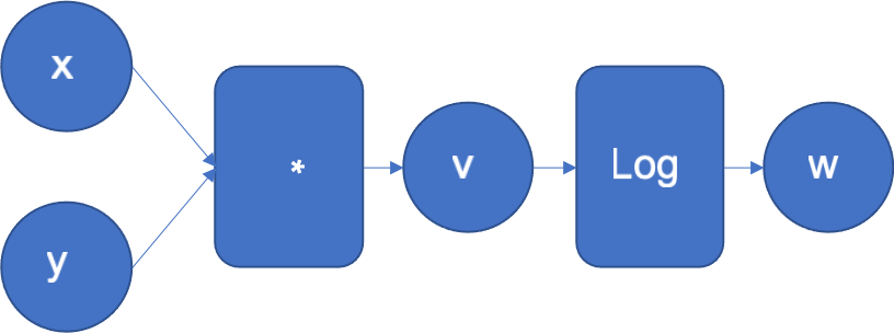
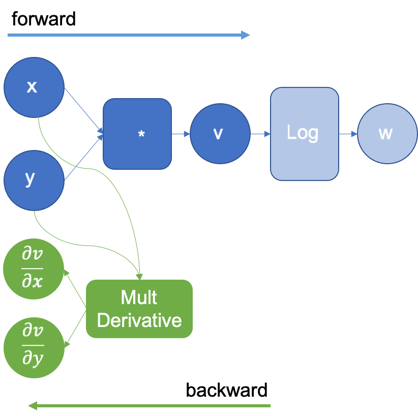
Let’s look at a very simple program that just computes an inverse and the gradient of that operation to show how autograd works:

t = torch.tensor(((1, 2), (3, 4)), dtype=torch.float32, requires_grad=True)

inv = torch.linalg.inv(t)
inv.backward(torch.ones_like(inv))

print(t.grad)
: tensor([[-0.5000, 0.5000],
          [ 0.5000, -0.5000]])

We can mimic the same computation in NumPy by defining the autograd formula ourselves:

a = np.array(((1, 2), (3, 4)), dtype=np.float32)

inv_np = np.linalg.inv(a)

def inv_backward(result, grad):
    return -(result.transpose(-2, -1) @ (grad @ result.transpose(-2, -1)))
grad_np = inv_backward(inv_np, np.ones_like(inv_np))

print(grad_np)
: [[-0.5 0.5]
   [ 0.5 -0.5]]

Of course, as programs become more complicated it’s convenient to have builtin autograd support, and PyTorch’s linear algebra module supports both real and complex autograd.

CUDA Support

Support for autograd and accelerators, like CUDA devices, is a core part of PyTorch. The torch.linalg module was developed with NVIDIA’s PyTorch and cuSOLVER teams, who helped optimize its performance on CUDA devices with the cuSOLVER, cuBLAS, and MAGMA libraries. These improvements make PyTorch’s CUDA linear algebra operations faster than ever. For example, let’s look at the performance of PyTorch 1.9’s torch.linalg.cholesky vs. PyTorch 1.8’s (now deprecated) torch.cholesky:

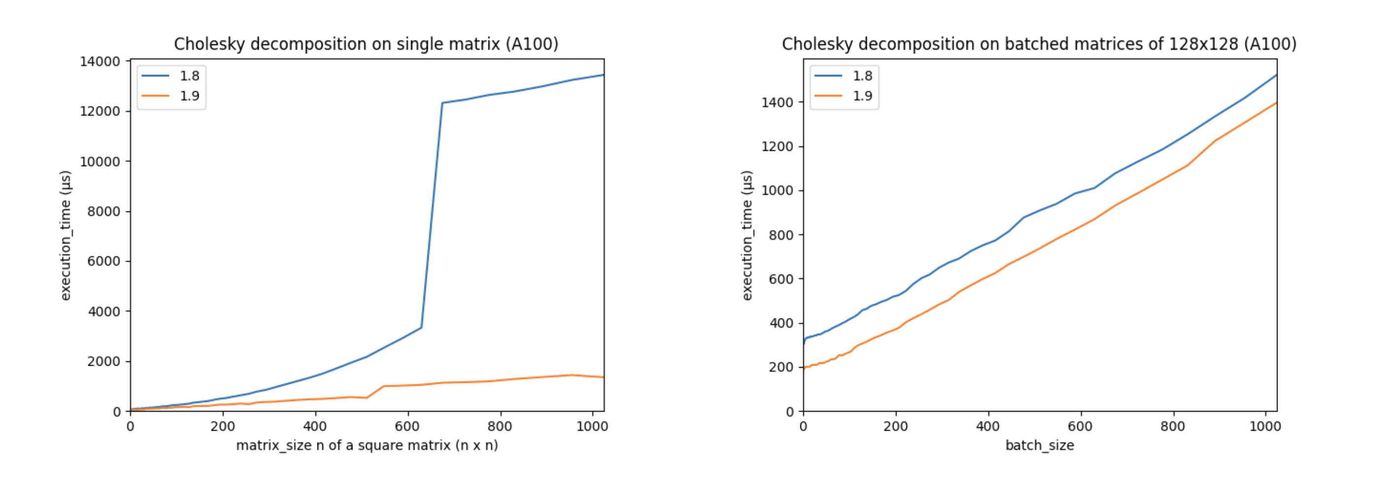
(The above charts were created using an Ampere A100 GPU with CUDA 11.3, cuSOLVER 11.1.1.58, and MAGMA 2.5.2. Matrices are in double precision.)

These charts show that performance has increased significantly on larger matrices, and that batched performance is better across the board. Other linear algebra operations, including torch.linalg.qr and torch.linalg.lstsq, have also had their CUDA performance improved.

Beyond NumPy

In addition to offering all the functions in NumPy’s linear algebra module with support for autograd and accelerators, torch.linalg has a few new functions of its own. NumPy’s linalg.norm does not allow users to compute vector norms over arbitrary subsets of dimensions, so to enable this functionality we added torch.linalg.vector_norm. We’ve also started modernizing other linear algebra functionality in PyTorch, so we created torch.linalg.householder_product to replace the older torch.orgqr, and we plan to continue adding more linear algebra functionality in the future, too.

The Future of Linear Algebra in PyTorch

The torch.linalg module is fast and familiar with great support for autograd and accelerators. It’s already being used in libraries like botorch, too. But we’re not stopping here. We plan to continue updating more of PyTorch’s existing linear algebra functionality (like torch.lobpcg) and offering more support for low rank and sparse linear algebra. We also want to hear your feedback on how we can improve, so start a conversation on the forum or file an issue on our Github and share your thoughts.

We look forward to hearing from you and seeing what the community does with PyTorch’s new linear algebra functionality!

Read More

An Overview of the PyTorch Mobile Demo Apps

PyTorch Mobile provides a runtime environment to execute state-of-the-art machine learning models on mobile devices. Latency is reduced, privacy preserved, and models can run on mobile devices anytime, anywhere.

In this blog post, we provide a quick overview of 10 currently available PyTorch Mobile powered demo apps running various state-of-the-art PyTorch 1.9 machine learning models spanning images, video, audio and text.

It’s never been easier to deploy a state-of-the-art ML model to a phone. You don’t need any domain knowledge in Machine Learning and we hope one of the below examples resonates enough with you to be the starting point for your next project.

Computer Vision

Image Classification

This app demonstrates how to use PyTorch C++ libraries on iOS and Android to classify a static image with the MobileNetv2/3 model.

iOS #1 iOS #2 Android #1 Android #2

iOS Android

Live Image Classification

This app demonstrates how to run a quantized MobileNetV2 and Resnet18 models to classify images in real time with an iOS and Android device camera.

iOS Android


Image Segmentation

This app demonstrates how to use the PyTorch DeepLabV3 model to segment images. The updated app for PyTorch 1.9 also demonstrates how to create the model using the Mobile Interpreter and load the model with the LiteModuleLoader API.

iOS Android

iOS Android

Vision Transformer for Handwritten Digit Recognition

This app demonstrates how to use Facebook’s latest optimized Vision Transformer DeiT model to do image classification and handwritten digit recognition.

iOS Android

Android

Object Detection

This app demonstrates how to convert the popular YOLOv5 model and use it on an iOS app that detects objects from pictures in your photos, taken with camera, or with live camera.

iOS Android

iOS Android

D2Go

This app demonstrates how to create and use a much lighter and faster Facebook D2Go model to detect objects from pictures in your photos, taken with camera, or with live camera.

iOS Android

iOS Android

Video

Video Classification

This app demonstrates how to use a pre-trained PyTorchVideo model to perform video classification on tested videos, videos from the Photos library, or even real-time videos.

iOS Android

iOS Android Deep Dive

Natural Language Processing

Text Classification

This app demonstrates how to use a pre-trained Reddit model to perform text classification.

iOS Android

Machine Translation

This app demonstrates how to convert a sequence-to-sequence neural machine translation model trained with the code in the PyTorch NMT tutorial for french to english translation.

iOS Android

iOS Android

Question Answering

This app demonstrates how to use the DistilBERT Hugging Face transformer model to answer questions about Pytorch Mobile itself.

iOS Android

iOS Android

Audio

Speech Recognition

This app demonstrates how to convert Facebook AI’s torchaudio-powered wav2vec 2.0, one of the leading models in speech recognition to TorchScript before deploying it.

iOS Android

We really hope one of these demo apps stood out for you. For the full list, make sure to visit the iOS and Android demo app repos. You should also definitely check out the video An Overview of the PyTorch Mobile Demo Apps which provides both an overview of the PyTorch mobile demo apps and a deep dive into the PyTorch Video app for iOS and Android.

Read More

Everything You Need To Know About Torchvision’s SSD Implementation

In TorchVision v0.10, we’ve released two new Object Detection models based on the SSD architecture. Our plan is to cover the key implementation details of the algorithms along with information on how they were trained in a two-part article.

In part 1 of the series, we will focus on the original implementation of the SSD algorithm as described on the Single Shot MultiBox Detector paper. We will briefly give a high-level description of how the algorithm works, then go through its main components, highlight key parts of its code, and finally discuss how we trained the released model. Our goal is to cover all the necessary details to reproduce the model including those optimizations which are not covered on the paper but are part on the original implementation.

How Does SSD Work?

Reading the aforementioned paper is highly recommended but here is a quick oversimplified refresher. Our target is to detect the locations of objects in an image along with their categories. Here is the Figure 5 from the SSD paper with prediction examples of the model:

The SSD algorithm uses a CNN backbone, passes the input image through it and takes the convolutional outputs from different levels of the network. The list of these outputs are called feature maps. These feature maps are then passed through the Classification and Regression heads which are responsible for predicting the class and the location of the boxes.

Since the feature maps of each image contain outputs from different levels of the network, their size varies and thus they can capture objects of different dimensions. On top of each, we tile several default boxes which can be thought as our rough prior guesses. For each default box, we predict whether there is an object (along with its class) and its offset (correction over the original location). During training time, we need to first match the ground truth to the default boxes and then we use those matches to estimate our loss. During inference, similar prediction boxes are combined to estimate the final predictions.

The SSD Network Architecture

In this section, we will discuss the key components of SSD. Our code follows closely the paper and makes use of many of the undocumented optimizations included in the official implementation.

DefaultBoxGenerator

The DefaultBoxGenerator class is responsible for generating the default boxes of SSD and operates similarly to the AnchorGenerator of FasterRCNN (for more info on their differences see pages 4-6 of the paper). It produces a set of predefined boxes of specific width and height which are tiled across the image and serve as the first rough prior guesses of where objects might be located. Here is Figure 1 from the SSD paper with a visualization of ground truths and default boxes:

The class is parameterized by a set of hyperparameters that control their shape and tiling. The implementation will provide automatically good guesses with the default parameters for those who want to experiment with new backbones/datasets but one can also pass optimized custom values.

SSDMatcher

The SSDMatcher class extends the standard Matcher used by FasterRCNN and it is responsible for matching the default boxes to the ground truth. After estimating the IoUs of all combinations, we use the matcher to find for each default box the best candidate ground truth with overlap higher than the IoU threshold. The SSD version of the matcher has an extra step to ensure that each ground truth is matched with the default box that has the highest overlap. The results of the matcher are used in the loss estimation during the training process of the model.

Classification and Regression Heads

The SSDHead class is responsible for initializing the Classification and Regression parts of the network. Here are a few notable details about their code:

Backbone Feature Extractor

The feature extractor reconfigures and enhances a standard VGG backbone with extra layers as depicted on the Figure 2 of the SSD paper:

The class supports all VGG models of TorchVision and one can create a similar extractor class for other types of CNNs (see this example for ResNet). Here are a few implementation details of the class:

  • Patching the ceil_mode parameter of the 3rd Maxpool layer is necessary to get the same feature map sizes as the paper. This is due to small differences between PyTorch and the original Caffe implementation of the model.
  • It adds a series of extra feature layerson top of VGG. If the highres parameter is True during its construction, it will append an extra convolution. This is useful for the SSD512 version of the model.
  • As discussed on section 3 of the paper, the fully connected layers of the original VGG are converted to convolutions with the first one using Atrous. Moreover maxpool5’s stride and kernel size is modified.
  • As described on section 3.1, L2 normalization is used on the output of conv4_3 and a set of learnable weights are introduced to control its scaling.

SSD Algorithm

The final key piece of the implementation is on the SSD class. Here are some notable details:

Here are the two core methods of the implementation:

The SSD300 VGG16 Model

The SSD is a family of models because it can be configured with different backbones and different Head configurations. In this section, we will focus on the provided SSD pre-trained model. We will discuss the details of its configuration and the training process used to reproduce the reported results.

Training process

The model was trained using the COCO dataset and all of its hyper-parameters and scripts can be found in our references folder. Below we provide details on the most notable aspects of the training process.

Paper Hyperparameters

In order to achieve the best possible results on COCO, we adopted the hyperparameters described on the section 3 of the paper concerning the optimizer configuration, the weight regularization etc. Moreover we found it useful to adopt the optimizations that appear in the official implementation concerning the tiling configuration of the DefaultBox generator. This optimization was not described in the paper but it was crucial for improving the detection precision of smaller objects.

Data Augmentation

Implementing the SSD Data Augmentation strategy as described on page 6 and page 12 of the paper was critical to reproducing the results. More specifically the use of random “Zoom In” and “Zoom Out” transformations make the model robust to various input sizes and improve its precision on the small and medium objects. Finally since the VGG16 has quite a few parameters, the photometric distortions included in the augmentations have a regularization effect and help avoid the overfitting.

Weight Initialization & Input Scaling

Another aspect that we found beneficial was to follow the weight initialization scheme proposed by the paper. To do that, we had to adapt our input scaling method by undoing the 0-1 scaling performed by ToTensor() and use pre-trained ImageNet weights fitted with this scaling (shoutout to Max deGroot for providing them in his repo). All the weights of new convolutions were initialized using Xavier and their biases were set to zero. After initialization, the network was trained end-to-end.

LR Scheme

As reported on the paper, after applying aggressive data augmentations it’s necessary to train the models for longer. Our experiments confirm this and we had to tweak the Learning rate, batch sizes and overall steps to achieve the best results. Our proposed learning scheme is configured to be rather on the safe side, showed signs of plateauing between the steps and thus one is likely to be able to train a similar model by doing only 66% of our epochs.

Breakdown of Key Accuracy Improvements

It is important to note that implementing a model directly from a paper is an iterative process that circles between coding, training, bug fixing and adapting the configuration until we match the accuracies reported on the paper. Quite often it also involves simplifying the training recipe or enhancing it with more recent methodologies. It is definitely not a linear process where incremental accuracy improvements are achieved by improving a single direction at a time but instead involves exploring different hypothesis, making incremental improvements in different aspects and doing a lot of backtracking.

With that in mind, below we try to summarize the optimizations that affected our accuracy the most. We did this by grouping together the various experiments in 4 main groups and attributing the experiment improvements to the closest match. Note that the Y-axis of the graph starts from 18 instead from 0 to make the difference between optimizations more visible:

Model Configuration mAP delta mAP
Baseline with “FasterRCNN-style” Hyperparams 19.5
+ Paper Hyperparams 1.6 21.1
+ Data Augmentation 1.8 22.9
+ Weight Initialization & Input Scaling 1 23.9
+ LR scheme 1.2 25.1

Our final model achieves an mAP of 25.1 and reproduces exactly the COCO results reported on the paper. Here is a detailed breakdown of the accuracy metrics.

We hope you found the part 1 of the series interesting. On the part 2, we will focus on the implementation of SSDlite and discuss its differences from SSD. Until then, we are looking forward to your feedback.

Read More

PyTorch 1.9 Release, including torch.linalg and Mobile Interpreter

We are excited to announce the release of PyTorch 1.9. The release is composed of more than 3,400 commits since 1.8, made by 398 contributors. The release notes are available here. Highlights include:

  1. Major improvements to support scientific computing, including torch.linalg, torch.special, and Complex Autograd
  2. Major improvements in on-device binary size with Mobile Interpreter
  3. Native support for elastic-fault tolerance training through the upstreaming of TorchElastic into PyTorch Core
  4. Major updates to the PyTorch RPC framework to support large scale distributed training with GPU support
  5. New APIs to optimize performance and packaging for model inference deployment
  6. Support for Distributed training, GPU utilization and SM efficiency in the PyTorch Profiler

Along with 1.9, we are also releasing major updates to the PyTorch libraries, which you can read about in this blog post.

We’d like to thank the community for their support and work on this latest release. We’d especially like to thank Quansight and Microsoft for their contributions.

Features in PyTorch releases are classified as Stable, Beta, and Prototype. You can learn more about the definitions in this blog post.

Frontend APIs

(Stable) torch.linalg

In 1.9, the torch.linalg module is moving to a stable release. Linear algebra is essential to deep learning and scientific computing, and the torch.linalg module extends PyTorch’s support for it with implementations of every function from NumPy’s linear algebra module (now with support for accelerators and autograd) and more, like torch.linalg.matrix_norm and torch.linalg.householder_product. This makes the module immediately familiar to users who have worked with NumPy. Refer to the documentation here.

We plan to publish another blog post with more details on the torch.linalg module next week!

(Stable) Complex Autograd

The Complex Autograd feature, released as a beta in PyTorch 1.8, is now stable. Since the beta release, we have extended support for Complex Autograd for over 98% operators in PyTorch 1.9, improved testing for complex operators by adding more OpInfos, and added greater validation through TorchAudio migration to native complex tensors (refer to this issue).

This feature provides users the functionality to calculate complex gradients and optimize real valued loss functions with complex variables. This is a required feature for multiple current and downstream prospective users of complex numbers in PyTorch like TorchAudio, ESPNet, Asteroid, and FastMRI. Refer to the documentation for more details.

(Stable) torch.use_deterministic_algorithms()

To help with debugging and writing reproducible programs, PyTorch 1.9 includes a torch.use_determinstic_algorithms option. When this setting is enabled, operations will behave deterministically, if possible, or throw a runtime error if they might behave nondeterministically. Here are a couple examples:

>>> a = torch.randn(100, 100, 100, device='cuda').to_sparse()
>>> b = torch.randn(100, 100, 100, device='cuda')

# Sparse-dense CUDA bmm is usually nondeterministic
>>> torch.bmm(a, b).eq(torch.bmm(a, b)).all().item()
False

>>> torch.use_deterministic_algorithms(True)

# Now torch.bmm gives the same result each time, but with reduced performance
>>> torch.bmm(a, b).eq(torch.bmm(a, b)).all().item()
True

# CUDA kthvalue has no deterministic algorithm, so it throws a runtime error
>>> torch.zeros(10000, device='cuda').kthvalue(1)
RuntimeError: kthvalue CUDA does not have a deterministic implementation...

PyTorch 1.9 adds deterministic implementations for a number of indexing operations, too, including index_add, index_copy, and index_put with accum=False. For more details, refer to the documentation and reproducibility note.

(Beta) torch.special

A torch.special module, analogous to SciPy’s special module, is now available in beta. This module contains many functions useful for scientific computing and working with distributions such as iv, ive, erfcx, logerfc, and logerfcx. Refer to the documentation for more details.

(Beta) nn.Module parameterization

nn.Module parameterization allows users to parametrize any parameter or buffer of an nn.Module without modifying the nn.Module itself. It allows you to constrain the space in which your parameters live without the need for special optimization methods.

This also contains a new implementation of the spectral_norm parametrization for PyTorch 1.9. More parametrization will be added to this feature (weight_norm, matrix constraints and part of pruning) for the feature to become stable in 1.10. For more details, refer to the documentation and tutorial.

PyTorch Mobile

(Beta) Mobile Interpreter

We are releasing Mobile Interpreter, a streamlined version of the PyTorch runtime, in beta. The Interpreter will execute PyTorch programs in edge devices, with reduced binary size footprint.

Mobile Interpreter is one of the top requested features for PyTorch Mobile. This new release will significantly reduce binary size compared with the current on-device runtime. In order for you to get the binary size improvements with our interpreter (which can reduce the binary size up to ~75% for a typical application) follow these instructions. As an example, using Mobile Interpreter, we can reach 2.6 MB compressed with MobileNetV2 in arm64-v7a Android. With this latest release we are making it much simpler to integrate the interpreter by providing pre-built libraries for iOS and Android.

TorchVision Library

Starting from 1.9, users can use the TorchVision library on their iOS/Android apps. The Torchvision library contains the C++ TorchVision ops and needs to be linked together with the main PyTorch library for iOS, for Android it can be added as a gradle dependency. This allows using TorchVision prebuilt MaskRCNN operators for object detections and segmentation. To learn more about the library, please refer to our tutorials and demo apps.

Demo apps

We are releasing a new video app based on PyTorch Video library and an updated speech recognition app based on the latest torchaudio, wave2vec model. Both are available on iOS and Android. In addition, we have updated the seven Computer Vision and three Natural Language Processing demo apps, including the HuggingFace DistilBERT, and the DeiT vision transformer models, with PyTorch Mobile v1.9. With the addition of these two apps, we now offer a full suite of demo apps covering image, text, audio, and video. To get started check out our iOS demo apps and Android demo apps.

Distributed Training

(Beta) TorchElastic is now part of core

TorchElastic, which was open sourced over a year ago in the pytorch/elastic github repository, is a runner and coordinator for PyTorch worker processes. Since then, it has been adopted by various distributed torch use-cases: 1) deepspeech.pytorch 2) pytorch-lightning 3) Kubernetes CRD. Now, it is part of PyTorch core.

As its name suggests, the core function of TorcheElastic is to gracefully handle scaling events. A notable corollary of elasticity is that peer discovery and rank assignment are built into TorchElastic enabling users to run distributed training on preemptible instances without requiring a gang scheduler. As a side note, etcd used to be a hard dependency of TorchElastic. With the upstream, this is no longer the case since we have added a “standalone” rendezvous based on c10d::Store. For more details, refer to the documentation.

(Beta) Distributed Training Updates

In addition to TorchElastic, there are a number of beta features available in the distributed package:

  • (Beta) CUDA support is available in RPC: Compared to CPU RPC and general-purpose RPC frameworks, CUDA RPC is a much more efficient way for P2P Tensor communication. It is built on top of TensorPipe which can automatically choose a communication channel for each Tensor based on Tensor device type and channel availability on both the caller and the callee. Existing TensorPipe channels cover NVLink, InfiniBand, SHM, CMA, TCP, etc. See this recipe for how CUDA RPC helps to attain 34x speedup compared to CPU RPC.

  • (Beta) ZeroRedundancyOptimizer: ZeroRedundancyOptimizer can be used in conjunction with DistributedDataParallel to reduce the size of per-process optimizer states. The idea of ZeroRedundancyOptimizer comes from DeepSpeed/ZeRO project and Marian, where the optimizer in each process owns a shard of model parameters and their corresponding optimizer states. When running step(), each optimizer only updates its own parameters, and then uses collective communication to synchronize updated parameters across all processes. Refer to this documentation and this tutorial to learn more.

  • (Beta) Support for profiling distributed collectives: PyTorch’s profiler tools, torch.profiler and torch.autograd.profiler, are able to profile distributed collectives and point to point communication primitives including allreduce, alltoall, allgather, send/recv, etc. This is enabled for all backends supported natively by PyTorch: gloo, mpi, and nccl. This can be used to debug performance issues, analyze traces that contain distributed communication, and gain insight into performance of applications that use distributed training. To learn more, refer to this documentation.

Performance Optimization and Tooling

(Stable) Freezing API

Module Freezing is the process of inlining module parameters and attributes values as constants into the TorchScript internal representation. This allows further optimization and specialization of your program, both for TorchScript optimizations and lowering to other backends. It is used by optimize_for_mobile API, ONNX, and others.

Freezing is recommended for model deployment. It helps TorchScript JIT optimizations optimize away overhead and bookkeeping that is necessary for training, tuning, or debugging PyTorch models. It enables graph fusions that are not semantically valid on non-frozen graphs – such as fusing Conv-BN. For more details, refer to the documentation.

(Beta) PyTorch Profiler

The new PyTorch Profiler graduates to beta and leverages Kineto for GPU profiling, TensorBoard for visualization and is now the standard across our tutorials and documentation.

PyTorch 1.9 extends support for the new torch.profiler API to more builds, including Windows and Mac and is recommended in most cases instead of the previous torch.autograd.profiler API. The new API supports existing profiler features, integrates with CUPTI library (Linux-only) to trace on-device CUDA kernels and provides support for long-running jobs, e.g.:

def trace_handler(p):
    output = p.key_averages().table(sort_by="self_cuda_time_total", row_limit=10)
    print(output)
    p.export_chrome_trace("/tmp/trace_" + str(p.step_num) + ".json")

with profile(
    activities=[ProfilerActivity.CPU, ProfilerActivity.CUDA],
    # schedule argument specifies the iterations on which the profiler is active
    schedule=torch.profiler.schedule(
        wait=1,
        warmup=1,
        active=2),
    # on_trace_ready argument specifies the handler for the traces
    on_trace_ready=trace_handler
) as p:
    for idx in range(8):
        model(inputs)
        # profiler will trace iterations 2 and 3, and then 6 and 7 (counting from zero)
        p.step()

More usage examples can be found on the profiler recipe page.

The PyTorch Profiler Tensorboard plugin has new features for:

  • Distributed Training summary view with communications overview for NCCL
  • GPU Utilization and SM Efficiency in Trace view and GPU operators view
  • Memory Profiling view
  • Jump to source when launched from Microsoft VSCode
  • Ability for load traces from cloud object storage systems

(Beta) Inference Mode API

Inference Mode API allows significant speed-up for inference workloads while remaining safe and ensuring no incorrect gradients can ever be computed. It offers the best possible performance when no autograd is required. For more details, refer to the documentation for inference mode itself and the documentation explaining when to use it and the difference with no_grad mode.

(Beta) torch.package

torch.package is a new way to package PyTorch models in a self-contained, stable format. A package will include both the model’s data (e.g. parameters, buffers) and its code (model architecture). Packaging a model with its full set of Python dependencies, combined with a description of a conda environment with pinned versions, can be used to easily reproduce training. Representing a model in a self-contained artifact will also allow it to be published and transferred throughout a production ML pipeline while retaining the flexibility of a pure-Python representation. For more details, refer to the documentation.

(Prototype) prepare_for_inference

prepare_for_inference is a new prototype feature that takes in a module and performs graph-level optimizations to improve inference performance, depending on the device. It is meant to be a PyTorch-native option that requires minimal changes to user’s workflows. For more details, see the documentation for the Torchscript version here or the FX version here.

(Prototype) Profile-directed typing in TorchScript

TorchScript has a hard requirement for source code to have type annotations in order for compilation to be successful. For a long time, it was only possible to add missing or incorrect type annotations through trial and error (i.e., by fixing the type-checking errors generated by torch.jit.script one by one), which was inefficient and time consuming. Now, we have enabled profile directed typing for torch.jit.script by leveraging existing tools like MonkeyType, which makes the process much easier, faster, and more efficient. For more details, refer to the documentation.

Thanks for reading. If you’re interested in these updates and want to join the PyTorch community, we encourage you to join the discussion forums and open GitHub issues. To get the latest news from PyTorch, follow us on Facebook, Twitter, Medium, YouTube, or LinkedIn.

Cheers!

Team PyTorch

Read More

New PyTorch Library Releases in PyTorch 1.9, including TorchVision, TorchAudio, and more

Today, we are announcing updates to a number of PyTorch libraries, alongside the PyTorch 1.9 release. The updates include new releases for the domain libraries including TorchVision, TorchText and TorchAudio. These releases, along with the PyTorch 1.9 release, include a number of new features and improvements that will provide a broad set of updates for the PyTorch community.

Some highlights include:

  • TorchVision – Added new SSD and SSDLite models, quantized kernels for object detection, GPU Jpeg decoding, and iOS support. See release notes here.
  • TorchAudio – Added wav2vec 2.0 model deployable in non-Python environments (including C++, Android, and iOS). Many performance improvements in lfilter, spectral operations, resampling. Added options for quality control in sampling (i.e. Kaiser window support). Initiated the migration of complex tensors operations. Improved autograd support. See release notes here.
  • TorchText – Added a new high-performance Vocab module that provides common functional APIs for NLP workflows. See release notes here.

We’d like to thank the community for their support and work on this latest release.

Features in PyTorch releases are classified as Stable, Beta, and Prototype. You can learn more about the definitions in this blog post.

TorchVision 0.10

(Stable) Quantized kernels for object detection

The forward pass of the nms and roi_align operators now support tensors with a quantized dtype, which can help lower the memory footprint of object detection models, particularly on mobile environments. For more details, refer to the documentation.

(Stable) Speed optimizations for Tensor transforms

The resize and flip transforms have been optimized and its runtime improved by up to 5x on the CPU.

(Stable) Documentation improvements

Significant improvements were made to the documentation. In particular, a new gallery of examples is available. These examples visually illustrate how each transform acts on an image, and also properly documents and illustrates the output of the segmentation models.

The example gallery will be extended in the future to provide more comprehensive examples and serve as a reference for common torchvision tasks. For more details, refer to the documentation.

(Beta) New models for detection

SSD and SSDlite are two popular object detection architectures that are efficient in terms of speed and provide good results for low resolution pictures. In this release, we provide implementations for the original SSD model with VGG16 backbone and for its mobile-friendly variant SSDlite with MobileNetV3-Large backbone.

The models were pre-trained on COCO train2017 and can be used as follows:

import torch
import torchvision

# Original SSD variant
x = [torch.rand(3, 300, 300), torch.rand(3, 500, 400)]
m_detector = torchvision.models.detection.ssd300_vgg16(pretrained=True)
m_detector.eval()
predictions = m_detector(x)

# Mobile-friendly SSDlite variant
x = [torch.rand(3, 320, 320), torch.rand(3, 500, 400)]
m_detector = torchvision.models.detection.ssdlite320_mobilenet_v3_large(pretrained=True)
m_detector.eval()
predictions = m_detector(x)

The following accuracies can be obtained on COCO val2017 (full results available in #3403 and #3757):

Model mAP mAP@50 mAP@75
SSD300 VGG16 25.1 41.5 26.2
SSDlite320 MobileNetV3-Large 21.3 34.3 22.1

For more details, refer to the documentation.

(Beta) JPEG decoding on the GPU

Decoding jpegs is now possible on GPUs with the use of nvjpeg, which should be readily available in your CUDA setup. The decoding time of a single image should be about 2 to 3 times faster than with libjpeg on CPU. While the resulting tensor will be stored on the GPU device, the input raw tensor still needs to reside on the host (CPU), because the first stages of the decoding process take place on the host:
from torchvision.io.image import read_file, decode_jpeg

data = read_file('path_to_image.jpg')  # raw data is on CPU
img = decode_jpeg(data, device='cuda')  # decoded image in on GPU

For more details, see the documentation.

(Beta) iOS support

TorchVision 0.10 now provides pre-compiled iOS binaries for its C++ operators, which means you can run Faster R-CNN and Mask R-CNN on iOS. An example app on how to build a program leveraging those ops can be found here.

TorchAudio 0.9.0

(Stable) Complex Tensor Migration

TorchAudio has functions that handle complex-valued tensors. These functions follow a convention to use an extra dimension to represent real and imaginary parts. In PyTorch 1.6, the native complex type was introduced. As its API is getting stable, torchaudio has started to migrate to the native complex type.

In this release, we added support for native complex tensors, and you can opt-in to use them. Using the native complex types, we have verified that affected functions continue to support autograd and TorchScript, moreover, switching to native complex types improves their performance. For more details, refer to pytorch/audio#1337.

(Stable) Filtering Improvement

In release 0.8, we added the C++ implementation of the core part of lfilter for CPU, which improved the performance. In this release, we optimized some internal operations of the CPU implementation for further performance improvement. We also added autograd support to both CPU and GPU. Now lfilter and all the biquad filters (biquad, band_biquad, bass_biquad, treble_biquad, allpass_biquad, lowpass_biquad, highpass_biquad, bandpass_biquad, equalizer_biquad and bandrefect_biquad) benefit from the performance improvement and support autograd. We also moved the implementation of overdrive to C++ for performance improvement. For more details, refer to the documentation.

(Stable) Improved Autograd Support

Along with the work of Complex Tensor Migration and Filtering Improvement, we also added autograd tests to transforms. lfilter, biquad and its variants, and most transforms are now guaranteed to support autograd. For more details, refer to the release note.

(Stable) Improved Windows Support

Torchaudio implements some operations in C++ for reasons such as performance and integration with third-party libraries. These C++ components were only available on Linux and macOS. In this release, we have added support to Windows. With this, the efficient filtering implementation mentioned above is also available on Windows.

However, please note that not all the C++ components are available for Windows. “sox_io” backend and torchaudio.functional.compute_kaldi_pitch are not supported.

(Stable) I/O Functions Migration

Since the 0.6 release, we have continuously improved I/O functionality. Specifically, in 0.8 we changed the default backend from “sox” to “sox_io” and applied the same switch to API of the “soundfile” backend. The 0.9 release concludes this migration by removing the deprecated backends. For more details, please refer to #903.

(Beta) Wav2Vec2.0 Model

We have added the model architectures from Wav2Vec2.0. You can import fine-tuned models parameters published on fairseq and Hugging Face Hub. Our model definition supports TorchScript, and it is possible to deploy the model to non-Python environments, such as C++, Android and iOS.

The following code snippet illustrates such a use case. Please check out our c++ example directory for the complete example. Currently, it is designed for running inference. If you would like more support for training, please file a feature request.

# Import fine-tuned model from Hugging Face Hub
import transformers
from torchaudio.models.wav2vec2.utils import import_huggingface_model

original = Wav2Vec2ForCTC.from_pretrained("facebook/wav2vec2-base-960h")
imported = import_huggingface_model(original)
# Import fine-tuned model from fairseq
import fairseq
from torchaudio.models.wav2vec2.utils import import_fairseq_model

original, _, _ = fairseq.checkpoint_utils.load_model_ensemble_and_task(
    ["wav2vec_small_960h.pt"], arg_overrides={'data': "<data_dir>"})
imported = import_fairseq_model(original[0].w2v_encoder)
# Build uninitialized model and load state dict
from torchaudio.models import wav2vec2_base

model = wav2vec2_base(num_out=32)
model.load_state_dict(imported.state_dict())

# Quantize / script / optimize for mobile
quantized_model = torch.quantization.quantize_dynamic(
    model, qconfig_spec={torch.nn.Linear}, dtype=torch.qint8)
scripted_model = torch.jit.script(quantized_model)
optimized_model = optimize_for_mobile(scripted_model)
optimized_model.save("model_for_deployment.pt")

For more details, see the documentation.

(Beta) Resampling Improvement

In release 0.8, we vectorized the operation in torchaudio.compliance.kaldi.resample_waveform, which improved the performance of resample_waveform and torchaudio.transforms.Resample. In this release, we have further revised the way the resampling algorithm is implemented.

We have:

  • Added Kaiser Window support for a wider range of resampling quality.
  • Added rolloff parameter for anti-aliasing control.
  • Added the mechanism to precompute the kernel and cache it in torchaudio.transforms.Resample for even faster operation.
  • Moved the implementation from torchaudio.compliance.kaldi.resample_waveform to torchaudio.functional.resample and deprecated torchaudio.compliance.kaldi.resample_waveform.

For more details, see the documentation.

(Prototype) RNN Transducer Loss

The RNN transducer loss is used in training RNN transducer models, which is a popular architecture for speech recognition tasks. The prototype loss in torchaudio currently supports autograd, torchscript, float16 and float32, and can also be run on both CPU and CUDA. For more details, please refer to the documentation.

TorchText 0.10.0

(Beta) New Vocab Module

In this release, we introduce a new Vocab module that replaces the current Vocab class. The new Vocab provides common functional APIs for NLP workflows. This module is backed by an efficient C++ implementation that reduces batch look-up time by up-to ~85% (refer to summary of #1248 and #1290 for further information on benchmarks), and provides support for TorchScript. We provide accompanying factory functions that can be used to build the Vocab object either through a python ordered dictionary or an Iterator that yields lists of tokens.

#creating Vocab from text file
import io
from torchtext.vocab import build_vocab_from_iterator
#generator that yield list of tokens
def yield_tokens(file_path):
   with io.open(file_path, encoding = 'utf-8') as f:
      for line in f:
          yield line.strip().split()
#get Vocab object
vocab_obj = build_vocab_from_iterator(yield_tokens(file_path), specials=["<unk>"])

#creating Vocab through ordered dict
from torchtext.vocab import vocab
from collections import Counter, OrderedDict
counter = Counter(["a", "a", "b", "b", "b"])
sorted_by_freq_tuples = sorted(counter.items(), key=lambda x: x[1], reverse=True)
ordered_dict = OrderedDict(sorted_by_freq_tuples)
vocab_obj = vocab(ordered_dict)

#common API usage

#look-up index
vocab_obj["a"]

#batch look-up indices
vocab_obj.looup_indices(["a","b"])
#support forward API of PyTorch nn Modules
vocab_obj(["a","b"])

#batch look-up tokens
vocab_obj.lookup_tokens([0,1])

#set default index to return when token not found
vocab_obj.set_default_index(0)
vocab_obj["out_of_vocabulary"] #prints 0

For more details, refer to the documentation.

Thanks for reading. If you’re interested in these updates and want to join the PyTorch community, we encourage you to join the discussion forums and open GitHub issues. To get the latest news from PyTorch, follow us on Facebook, Twitter, Medium, YouTube or LinkedIn.

Cheers!

-Team PyTorch

Read More

Overview of PyTorch Autograd Engine

This blog post is based on PyTorch version 1.8, although it should apply for older versions too, since most of the mechanics have remained constant.

To help understand the concepts explained here, it is recommended that you read the awesome blog post by @ezyang: PyTorch internals if you are not familiar with PyTorch architecture components such as ATen or c10d.

What is autograd?

Background

PyTorch computes the gradient of a function with respect to the inputs by using automatic differentiation. Automatic differentiation is a technique that, given a computational graph, calculates the gradients of the inputs. Automatic differentiation can be performed in two different ways; forward and reverse mode. Forward mode means that we calculate the gradients along with the result of the function, while reverse mode requires us to evaluate the function first, and then we calculate the gradients starting from the output. While both modes have their pros and cons, the reverse mode is the de-facto choice since the number of outputs is smaller than the number of inputs, which allows a much more efficient computation. Check [3] to learn more about this.

Automatic differentiation relies on a classic calculus formula known as the chain-rule. The chain rule allows us to calculate very complex derivatives by splitting them and recombining them later.

Formally speaking, given a composite function , we can calculate its derivative as . This result is what makes automatic differentiation work.
By combining the derivatives of the simpler functions that compose a larger one, such as a neural network, it is possible to compute the exact value of the gradient at a given point rather than relying on the numerical approximation, which would require multiple perturbations in the input to obtain a value.

To get the intuition of how the reverse mode works, let’s look at a simple function . Figure 1 shows its computational graph where the inputs x, y in the left, flow through a series of operations to generate the output z.

Figure 1: Computational graph of f(x, y) = log(x*y)

The automatic differentiation engine will normally execute this graph. It will also extend it to calculate the derivatives of w with respect to the inputs x, y, and the intermediate result v.

The example function can be decomposed in f and g, where and . Every time the engine executes an operation in the graph, the derivative of that operation is added to the graph to be executed later in the backward pass. Note, that the engine knows the derivatives of the basic functions.

In the example above, when multiplying x and y to obtain v, the engine will extend the graph to calculate the partial derivatives of the multiplication by using the multiplication derivative definition that it already knows. and . The resulting extended graph is shown in Figure 2, where the MultDerivative node also calculates the product of the resulting gradients by an input gradient to apply the chain rule; this will be explicitly seen in the following operations. Note that the backward graph (green nodes) will not be executed until all the forward steps are completed.

Figure 2: Computational graph extended after executing the logarithm

Continuing, the engine now calculates the operation and extends the graph again with the log derivative that it knows to be . This is shown in figure 3. This operation generates the result that when propagated backward and multiplied by the multiplication derivative as in the chain rule, generates the derivatives , .

Figure 3: Computational graph extended after executing the logarithm

The original computation graph is extended with a new dummy variable z that is the same w. The derivative of z with respect to w is 1 as they are the same variable, this trick allows us to apply the chain rule to calculate the derivatives of the inputs. After the forward pass is complete, we start the backward pass, by supplying the initial value of 1.0 for . This is shown in Figure 4.

Figure 4: Computational graph extended for reverse auto differentiation

Then following the green graph we execute the LogDerivative operation that the auto differentiation engine introduced, and multiply its result by to obtain the gradient as per the chain rule states. Next, the multiplication derivative is executed in the same way, and the desired derivatives are finally obtained.

Formally, what we are doing here, and PyTorch autograd engine also does, is computing a Jacobian-vector product (Jvp) to calculate the gradients of the model parameters, since the model parameters and inputs are vectors.

The Jacobian-vector product

When we calculate the gradient of a vector-valued function (a function whose inputs and outputs are vectors), we are essentially constructing a Jacobian matrix .

Thanks to the chain rule, multiplying the Jacobian matrix of a function by a vector with the previously calculated gradients of a scalar function results in the gradients of the scalar output with respect to the vector-valued function inputs.

As an example, let’s look at some functions in python notation to show how the chain rule applies.

def f(x1, x2):
      a = x1 * x2
      y1 = log(a)
      y2 = sin(x2)
      return (y1, y2)
  

def g(y1, y2):
      return y1 * y2
  

Now, if we derive this by hand using the chain rule and the definition of the derivatives, we obtain the following set of identities that we can directly plug into the Jacobian matrix of

Next, let’s consider the gradients for the scalar function

If we now calculate the transpose-Jacobian vector product obeying the chain rule, we obtain the following expression:

Evaluating the Jvp for yields the result:

We can execute the same expression in PyTorch and calculate the gradient of the input:

>>> import torch
>>> x = torch.tensor([0.5, 0.75], requires_grad=True)
>>> y = torch.log(x[0] * x[1]) * torch.sin(x[1])
>>> y.backward(1.0)
>>> x.grad

tensor([1.3633,
0.1912])</pre>

The result is the same as our hand-calculated Jacobian-vector product!
However, PyTorch never constructed the matrix as it could grow prohibitively large but instead, created a graph of operations that traversed backward while applying the Jacobian-vector products defined in tools/autograd/derivatives.yaml.

Going through the graph

Every time PyTorch executes an operation, the autograd engine constructs the graph to be traversed backward.
The reverse mode auto differentiation starts by adding a scalar variable at the end so that as we saw in the introduction. This is the initial gradient value that is supplied to the Jvp engine calculation as we saw in the section above.

In PyTorch, the initial gradient is explicitly set by the user when he calls the backward method.

Then, the Jvp calculation starts but it never constructs the matrix. Instead, when PyTorch records the computational graph, the derivatives of the executed forward operations are added (Backward Nodes). Figure 5 shows a backward graph generated by the execution of the functions and seen before.

Figure 5: Computational Graph extended with the backward pass

Once the forward pass is done, the results are used in the backward pass where the derivatives in the computational graph are executed. The basic derivatives are stored in the tools/autograd/derivatives.yaml file and they are not regular derivatives but the Jvp versions of them [3]. They take their primitive function inputs and outputs as parameters along with the gradient of the function outputs with respect to the final outputs. By repeatedly multiplying the resulting gradients by the next Jvp derivatives in the graph, the gradients up to the inputs will be generated following the chain rule.

Figure 6: How the chain rule is applied in backward differentiation

Figure 6 represents the process by showing the chain rule. We started with a value of 1.0 as detailed before which is the already calculated gradient highlighted in green. And we move to the next node in the graph. The backward function registered in derivatives.yaml will calculate the associated
value highlighted in red and multiply it by . By the chain rule this results in which will be the already calculated gradient (green) when we process the next backward node in the graph.

You may also have noticed that in Figure 5 there is a gradient generated from two different sources. When two different functions share an input, the gradients with respect to the output are aggregated for that input, and calculations using that gradient can’t proceed unless all the paths have been aggregated together.

Let’s see an example of how the derivatives are stored in PyTorch.

Suppose that we are currently processing the backward propagation of the function, in the LogBackward node in Figure 2. The derivative of in derivatives.yaml is specified as grad.div(self.conj()). grad is the already calculated gradient and self.conj() is the complex conjugate of the input vector. For complex numbers PyTorch calculates a special derivative called the conjugate Wirtinger derivative [6]. This derivative takes the complex number and its conjugate and by operating some magic that is described in [6], they are the direction of steepest descent when plugged into optimizers.

This code translates to , the corresponding green, and red squares in Figure 3. Continuing, the autograd engine will execute the next operation; backward of the multiplication. As before, the inputs are the original function’s inputs and the gradient calculated from the backward step. This step will keep repeating until we reach the gradient with respect to the inputs and the computation will be finished. The gradient of is only completed once the multiplication and sin gradients are added together. As you can see, we computed the equivalent of the Jvp but without constructing the matrix.

In the next post we will dive inside PyTorch code to see how this graph is constructed and where are the relevant pieces should you want to experiment with it!

References

  1. https://pytorch.org/tutorials/beginner/blitz/autograd_tutorial.html
  2. https://web.stanford.edu/class/cs224n/readings/gradient-notes.pdf
  3. https://www.cs.toronto.edu/~rgrosse/courses/csc321_2018/slides/lec10.pdf
  4. https://mustafaghali11.medium.com/how-pytorch-backward-function-works-55669b3b7c62
  5. https://indico.cern.ch/event/708041/contributions/3308814/attachments/1813852/2963725/automatic_differentiation_and_deep_learning.pdf
  6. https://pytorch.org/docs/stable/notes/autograd.html#complex-autograd-doc
  7. Recommended: shows why the backprop is formally expressed with the Jacobian

  8. cs.ubc.ca/~fwood/CS340/lectures/AD1.pdf

Read More

Everything you need to know about TorchVision’s MobileNetV3 implementation

In TorchVision v0.9, we released a series of new mobile-friendly models that can be used for Classification, Object Detection and Semantic Segmentation. In this article, we will dig deep into the code of the models, share notable implementation details, explain how we configured and trained them, and highlight important tradeoffs we made during their tuning. Our goal is to disclose technical details that typically remain undocumented in the original papers and repos of the models.

Network Architecture

The implementation of the MobileNetV3 architecture follows closely the original paper. It is customizable and offers different configurations for building Classification, Object Detection and Semantic Segmentation backbones. It was designed to follow a similar structure to MobileNetV2 and the two share common building blocks.

Off-the-shelf, we offer the two variants described on the paper: the Large and the Small. Both are constructed using the same code with the only difference being their configuration which describes the number of blocks, their sizes, their activation functions etc.

Configuration parameters

Even though one can write a custom InvertedResidual setting and pass it to the MobileNetV3 class directly, for the majority of applications we can adapt the existing configs by passing parameters to the model building methods. Some of the key configuration parameters are the following:

  • The width_mult parameter is a multiplier that affects the number of channels of the model. The default value is 1 and by increasing or decreasing it one can change the number of filters of all convolutions, including the ones of the first and last layers. The implementation ensures that the number of filters is always a multiple of 8. This is a hardware optimization trick which allows for faster vectorization of operations.

  • The reduced_tail parameter halves the number of channels on the last blocks of the network. This version is used by some Object Detection and Semantic Segmentation models. It’s a speed optimization which is described on the MobileNetV3 paper and reportedly leads to a 15% latency reduction without a significant negative effect on accuracy.

  • The dilated parameter affects the last 3 InvertedResidual blocks of the model and turns their normal depthwise Convolutions to Atrous Convolutions. This is used to control the output stride of these blocks and has a significant positive effect on the accuracy of Semantic Segmentation models.

Implementation details

Below we provide additional information on some notable implementation details of the architecture.
The MobileNetV3 class is responsible for building a network out of the provided configuration. Here are some implementation details of the class:

  • The last convolution block expands the output of the last InvertedResidual block by a factor of 6. The implementation is aligned with the Large and Small configurations described on the paper and can adapt to different values of the multiplier parameter.

  • Similarly to other models such as MobileNetV2, a dropout layer is placed just before the final Linear layer of the classifier.

The InvertedResidual class is the main building block of the network. Here are some notable implementation details of the block along with its visualization which comes from Figure 4 of the paper:

  • There is no expansion step if the input channels and the expanded channels are the same. This happens on the first convolution block of the network.

  • There is always a projection step even when the expanded channels are the same as the output channels.

  • The activation method of the depthwise block is placed before the Squeeze-and-Excite layer as this improves marginally the accuracy.

Classification

In this section we provide benchmarks of the pre-trained models and details on how they were configured, trained and quantized.

Benchmarks

Here is how to initialize the pre-trained models:

large = torchvision.models.mobilenet_v3_large(pretrained=True, width_mult=1.0,  reduced_tail=False, dilated=False)
small = torchvision.models.mobilenet_v3_small(pretrained=True)
quantized = torchvision.models.quantization.mobilenet_v3_large(pretrained=True)

Below we have the detailed benchmarks between new and selected previous models. As we can see MobileNetV3-Large is a viable replacement of ResNet50 for users who are willing to sacrifice a bit of accuracy for a roughly 6x speed-up:

Model Acc@1 Acc@5 Inference on CPU (sec) # Params (M)
MobileNetV3-Large 74.042 91.340 0.0411 5.48
MobileNetV3-Small 67.668 87.402 0.0165 2.54
Quantized MobileNetV3-Large 73.004 90.858 0.0162 2.96
MobileNetV2 71.880 90.290 0.0608 3.50
ResNet50 76.150 92.870 0.2545 25.56
ResNet18 69.760 89.080 0.1032 11.69

Note that the inference times are measured on CPU. They are not absolute benchmarks, but they allow for relative comparisons between models.

Training process

All pre-trained models are configured with a width multiplier of 1, have full tails, are non-dilated, and were fitted on ImageNet. Both the Large and Small variants were trained using the same hyper-parameters and scripts which can be found in our references folder. Below we provide details on the most notable aspects of the training process.

Achieving fast and stable training

Configuring RMSProp correctly was crucial to achieve fast training with numerical stability. The authors of the paper used TensorFlow in their experiments and in their runs they reported using quite high rmsprop_epsilon comparing to the default. Typically this hyper-parameter takes small values as it’s used to avoid zero denominators, but in this specific model choosing the right value seems important to avoid numerical instabilities in the loss.

Another important detail is that though PyTorch’s and TensorFlow’s RMSProp implementations typically behave similarly, there are a few differences with the most notable in our setup being how the epsilon hyperparameter is handled. More specifically, PyTorch adds the epsilon outside of the square root calculation while TensorFlow adds it inside. The result of this implementation detail is that one needs to adjust the epsilon value while porting the hyper parameter of the paper. A reasonable approximation can be taken with the formula PyTorch_eps = sqrt(TF_eps).

Increasing our accuracy by tuning hyperparameters & improving our training recipe

After configuring the optimizer to achieve fast and stable training, we turned into optimizing the accuracy of the model. There are a few techniques that helped us achieve this. First of all, to avoid overfitting we augmented out data using the AutoAugment algorithm, followed by RandomErasing. Additionally we tuned parameters such as the weight decay using cross validation. We also found beneficial to perform weight averaging across different epoch checkpoints after the end of the training. Finally, though not used in our published training recipe, we found that using Label Smoothing, Stochastic Depth and LR noise injection improve the overall accuracy by over 1.5 points.

The graph and table depict a simplified summary of the most important iterations for improving the accuracy of the MobileNetV3 Large variant. Note that the actual number of iterations done while training the model was significantly larger and that the progress in accuracy was not always monotonically increasing. Also note that the Y-axis of the graph starts from 70% instead from 0% to make the difference between iterations more visible:

Iteration Acc@1 Acc@5
Baseline with “MobileNetV2-style” Hyperparams 71.542 90.068
+ RMSProp with default eps 70.684 89.38
+ RMSProp with adjusted eps & LR scheme 71.764 90.178
+ Data Augmentation & Tuned Hyperparams 73.86 91.292
+ Checkpoint Averaging 74.028 91.382
+ Label Smoothing & Stochastic Depth & LR noise 75.536 92.368

Note that once we’ve achieved an acceptable accuracy, we verified the model performance on the hold-out test dataset which hasn’t been used before for training or hyper-parameter tuning. This process helps us detect overfitting and is always performed for all pre-trained models prior their release.

Quantization

We currently offer quantized weights for the QNNPACK backend of the MobileNetV3-Large variant which provides a speed-up of 2.5x. To quantize the model, Quantized Aware Training (QAT) was used. The hyper parameters and the scripts used to train the model can be found in our references folder.

Note that QAT allows us to model the effects of quantization and adjust the weights so that we can improve the model accuracy. This translates to an accuracy increase of 1.8 points comparing to simple post-training quantization:

Quantization Status Acc@1 Acc@5
Non-quantized 74.042 91.340
Quantized Aware Training 73.004 90.858
Post-training Quantization 71.160 89.834

Object Detection

In this section, we will first provide benchmarks of the released models, and then discuss how the MobileNetV3-Large backbone was used in a Feature Pyramid Network along with the FasterRCNN detector to perform Object Detection. We will also explain how the network was trained and tuned alongside with any tradeoffs we had to make. We will not cover details about how it was used with SSDlite as this will be discussed on a future article.

Benchmarks

Here is how the models are initialized:

high_res = torchvision.models.detection.fasterrcnn_mobilenet_v3_large_fpn(pretrained=T low_res = torchvision.models.detection.fasterrcnn_mobilenet_v3_large_320_fpn(pretraine

Below are some benchmarks between new and selected previous models. As we can see the high resolution Faster R-CNN with MobileNetV3-Large FPN backbone seems a viable replacement of the equivalent ResNet50 model for those users who are willing to sacrifice few accuracy points for a 5x speed-up:

Model mAP Inference on CPU (sec) # Params (M)
Faster R-CNN MobileNetV3-Large FPN (High-Res) 32.8 0.8409 19.39
Faster R-CNN MobileNetV3-Large 320 FPN (Low-Res) 22.8 0.1679 19.39
Faster R-CNN ResNet-50 FPN 37.0 4.1514 41.76
RetinaNet ResNet-50 FPN 36.4 4.8825 34.01

Implementation details

The Detector uses a FPN-style backbone which extracts features from different convolutions of the MobileNetV3 model. By default the pre-trained model uses the output of the 13th InvertedResidual block and the output of the Convolution prior to the pooling layer but the implementation supports using the outputs of more stages.

All feature maps extracted from the network have their output projected down to 256 channels by the FPN block as this greatly improves the speed of the network. These feature maps provided by the FPN backbone are used by the FasterRCNN detector to provide box and class predictions at different scales.

Training & Tuning process

We currently offer two pre-trained models capable of doing object detection at different resolutions. Both models were trained on the COCO dataset using the same hyper-parameters and scripts which can be found in our references folder.

The High Resolution detector was trained with images of 800-1333px, while the mobile-friendly Low Resolution detector was trained with images of 320-640px. The reason why we provide two separate sets of pre-trained weights is because training a detector directly on the smaller images leads to a 5 mAP increase in precision comparing to passing small images to the pre-trained high-res model. Both backbones were initialized with weights fitted on ImageNet and the 3 last stages of their weights where fined-tuned during the training process.

An additional speed optimization can be applied on the mobile-friendly model by tuning the RPN NMS thresholds. By sacrificing only 0.2 mAP of precision we were able to improve the CPU speed of the model by roughly 45%. The details of the optimization can be seen below:

Tuning Status mAP Inference on CPU (sec)
Before 23.0 0.2904
After 22.8 0.1679

Below we provide some examples of visualizing the predictions of the Faster R-CNN MobileNetV3-Large FPN model:

Semantic Segmentation

In this section we will start by providing some benchmarks of the released pre-trained models. Then we will discuss how a MobileNetV3-Large backbone was combined with segmentation heads such as LR-ASPP, DeepLabV3 and the FCN to conduct Semantic Segmentation. We will also explain how the network was trained and propose a few optional optimization techniques for speed critical applications.

Benchmarks

This is how to initialize the pre-trained models:

lraspp = torchvision.models.segmentation.lraspp_mobilenet_v3_large(pretrained=True) deeplabv3 = torchvision.models.segmentation.deeplabv3_mobilenet_v3_large(pretrained=Tr

Below are the detailed benchmarks between new and selected existing models. As we can see, the DeepLabV3 with a MobileNetV3-Large backbone is a viable replacement of FCN with ResNet50 for the majority of applications as it achieves similar accuracy with a 8.5x speed-up. We also observe that the LR-ASPP network supersedes the equivalent FCN in all metrics:

Model mIoU Global Pixel Acc Inference on CPU (sec) # Params (M)
LR-ASPP MobileNetV3-Large 57.9 91.2 0.3278 3.22
DeepLabV3 MobileNetV3-Large 60.3 91.2 0.5869 11.03
FCN MobileNetV3-Large (not released) 57.8 90.9 0.3702 5.05
DeepLabV3 ResNet50 66.4 92.4 6.3531 39.64
FCN ResNet50 60.5 91.4 5.0146 32.96

Implementation details

In this section we will discuss important implementation details of tested segmentation heads. Note that all models described in this section use a dilated MobileNetV3-Large backbone.

LR-ASPP

The LR-ASPP is the Lite variant of the Reduced Atrous Spatial Pyramid Pooling model proposed by the authors of the MobileNetV3 paper. Unlike the other segmentation models in TorchVision, it does not make use of an auxiliary loss. Instead it uses low and high-level features with output strides of 8 and 16 respectively.

Unlike the paper where a 49×49 AveragePooling layer with variable strides is used, our implementation uses an AdaptiveAvgPool2d layer to process the global features. This is because the authors of the paper tailored the head to the Cityscapes dataset while our focus is to provide a general purpose implementation that can work on multiple datasets. Finally our implementation always has a bilinear interpolation before returning the output to ensure that the sizes of the input and output images match exactly.

DeepLabV3 & FCN

The combination of MobileNetV3 with DeepLabV3 and FCN follows closely the ones of other models and the stage estimation for these methods is identical to LR-ASPP. The only notable difference is that instead of using high and low level features, we attach the normal loss to the feature map with output stride 16 and an auxiliary loss on the feature map with output stride 8.

Finally we should note that the FCN version of the model was not released because it was completely superseded by the LR-ASPP both in terms of speed and accuracy. The pre-trained weights are still available and can be used with minimal changes to the code.

Training & Tuning process

We currently offer two MobileNetV3 pre-trained models capable of doing semantic segmentation: the LR-ASPP and the DeepLabV3. The backbones of the models were initialized with ImageNet weights and trained end-to-end. Both architectures were trained on the COCO dataset using the same scripts with similar hyper-parameters. Their details can be found in our references folder.

Normally, during inference the images are resized to 520 pixels. An optional speed optimization is to construct a Low Res configuration of the model by using the High-Res pre-trained weights and reducing the inference resizing to 320 pixels. This will improve the CPU execution times by roughly 60% while sacrificing a couple of mIoU points. The detailed numbers of this optimization can be found on the table below:

Low-Res Configuration mIoU Difference Speed Improvement mIoU Global Pixel Acc Inference on CPU (sec)
LR-ASPP MobileNetV3-Large -2.1 65.26% 55.8 90.3 0.1139
DeepLabV3 MobileNetV3-Large -3.8 63.86% 56.5 90.3 0.2121
FCN MobileNetV3-Large (not released) -3.0 57.57% 54.8 90.1 0.1571

Here are some examples of visualizing the predictions of the LR-ASPP MobileNetV3-Large model:

We hope that you found this article interesting. We are looking forward to your feedback to see if this is the type of content you would like us to publish more often. If the community finds that such posts are useful, we will be happy to publish more articles that cover the implementation details of newly introduced Machine Learning models.

Read More

Announcing the PyTorch Enterprise Support Program

Today, we are excited to announce the PyTorch Enterprise Support Program, a participatory program that enables service providers to develop and offer tailored enterprise-grade support to their customers. This new offering, built in collaboration between Facebook and Microsoft, was created in direct response to feedback from PyTorch enterprise users who are developing models in production at scale for mission-critical applications.

The PyTorch Enterprise Support Program is available to any service provider. It is designed to mutually benefit all program Participants by sharing and improving PyTorch long-term support (LTS), including contributions of hotfixes and other improvements found while working closely with customers and on their systems.

To benefit the open source community, all hotfixes developed by Participants will be tested and fed back to the LTS releases of PyTorch regularly through PyTorch’s standard pull request process. To participate in the program, a service provider must apply and meet a set of program terms and certification requirements. Once accepted, the service provider becomes a program Participant and can offer a packaged PyTorch Enterprise support service with LTS, prioritized troubleshooting, useful integrations, and more.

As one of the founding members and an inaugural member of the PyTorch Enterprise Support Program, Microsoft is launching PyTorch Enterprise on Microsoft Azure to deliver a reliable production experience for PyTorch users. Microsoft will support each PyTorch release for as long as it is current. In addition, it will support selected releases for two years, enabling a stable production experience. Microsoft Premier and Unified Support customers can access prioritized troubleshooting for hotfixes, bugs, and security patches at no additional cost. Microsoft will extensively test PyTorch releases for performance regression. The latest release of PyTorch will be integrated with Azure Machine Learning and other PyTorch add-ons including ONNX Runtime for faster inference.

PyTorch Enterprise on Microsoft Azure not only benefits its customers, but also the PyTorch community users. All improvements will be tested and fed back to the future release for PyTorch so everyone in the community can use them.

As an organization or PyTorch user, the standard way of researching and deploying with different release versions of PyTorch does not change. If your organization is looking for the managed long-term support, prioritized patches, bug fixes, and additional enterprise-grade support, then you should reach out to service providers participating in the program.

To learn more and participate in the program as a service provider, visit the PyTorch Enterprise Support Program. If you want to learn more about Microsoft’s offering, visit PyTorch Enterprise on Microsoft Azure.

Thank you,

Team PyTorch

Read More

PyTorch Ecosystem Day 2021 Recap and New Contributor Resources

Thank you to our incredible community for making the first ever PyTorch Ecosystem Day a success! The day was filled with discussions on new developments, trends and challenges showcased through 71 posters, 32 breakout sessions and 6 keynote speakers.

Special thanks to our keynote speakers: Piotr Bialecki, Ritchie Ng, Miquel Farré, Joe Spisak, Geeta Chauhan, and Suraj Subramanian who shared updates from the latest release of PyTorch, exciting work being done with partners, use case example from Disney, the growth and development of the PyTorch community in Asia Pacific, and latest contributor highlights.

If you missed the opening talks, you rewatch them here:

In addition to the talks, we had 71 posters covering various topics such as multimodal, NLP, compiler, distributed training, researcher productivity tools, AI accelerators, and more. From the event, it was clear that an underlying thread that ties all of these different projects together is the cross-collaboration of the PyTorch community. Thank you for continuing to push the state of the art with PyTorch!

To view the full catalogue of poster, please visit PyTorch Ecosystem Day 2021 Event Page.

New Contributor Resources

Today, we are also sharing new contributor resources that we are trying out to give you the most access to up-to-date news, networking opportunities and more.

  • Contributor Newsletter – Includes curated news including RFCs, feature roadmaps, notable PRs, editorials from developers, and more to support keeping track of everything that’s happening in our community.
  • Contributors Discussion Forum – Designed for contributors to learn and collaborate on the latest development across PyTorch.
  • PyTorch Developer Podcast (Beta) – Edward Yang, PyTorch Research Scientist, at Facebook AI shares bite-sized (10 to 20 mins) podcast episodes discussing topics about all sorts of internal development topics in PyTorch.

Thank you,

Team PyTorch

Read More

An overview of the ML models introduced in TorchVision v0.9

TorchVision v0.9 has been released and it is packed with numerous new Machine Learning models and features, speed improvements and bug fixes. In this blog post, we provide a quick overview of the newly introduced ML models and discuss their key features and characteristics.

Classification

  • MobileNetV3 Large & Small: These two classification models are optimized for Mobile use-cases and are used as backbones on other Computer Vision tasks. The implementation of the new MobileNetV3 architecture supports the Large & Small variants and the depth multiplier parameter as described in the original paper. We offer pre-trained weights on ImageNet for both Large and Small networks with depth multiplier 1.0 and resolution 224×224. Our previous training recipes have been updated and can be used to easily train the models from scratch (shoutout to Ross Wightman for inspiring some of our training configuration). The Large variant offers a competitive accuracy comparing to ResNet50 while being over 6x faster on CPU, meaning that it is a good candidate for applications where speed is important. For applications where speed is critical, one can sacrifice further accuracy for speed and use the Small variant which is 15x faster than ResNet50.

  • Quantized MobileNetV3 Large: The quantized version of MobilNetV3 Large reduces the number of parameters by 45% and it is roughly 2.5x faster than the non-quantized version while remaining competitive in terms of accuracy. It was fitted on ImageNet using Quantization Aware Training by iterating on the non-quantized version and it can be trained from scratch using the existing reference scripts.

Usage:

model = torchvision.models.mobilenet_v3_large(pretrained=True)
# model = torchvision.models.mobilenet_v3_small(pretrained=True)
# model = torchvision.models.quantization.mobilenet_v3_large(pretrained=True)
model.eval()
predictions = model(img)

Object Detection

  • Faster R-CNN MobileNetV3-Large FPN: Combining the MobileNetV3 Large backbone with a Faster R-CNN detector and a Feature Pyramid Network leads to a highly accurate and fast object detector. The pre-trained weights are fitted on COCO 2017 using the provided reference scripts and the model is 5x faster on CPU than the equivalent ResNet50 detector while remaining competitive in terms of accuracy.
  • Faster R-CNN MobileNetV3-Large 320 FPN: This is an iteration of the previous model that uses reduced resolution (min_size=320 pixel) and sacrifices accuracy for speed. It is 25x faster on CPU than the equivalent ResNet50 detector and thus it is good for real mobile use-cases.

Usage:

model = torchvision.models.detection.fasterrcnn_mobilenet_v3_large_fpn(pretrained=True)
# model = torchvision.models.detection.fasterrcnn_mobilenet_v3_large_320_fpn(pretrained=True)
model.eval()
predictions = model(img)

Semantic Segmentation

  • DeepLabV3 with Dilated MobileNetV3 Large Backbone: A dilated version of the MobileNetV3 Large backbone combined with DeepLabV3 helps us build a highly accurate and fast semantic segmentation model. The pre-trained weights are fitted on COCO 2017 using our standard training recipes. The final model has the same accuracy as the FCN ResNet50 but it is 8.5x faster on CPU and thus making it an excellent replacement for the majority of applications.
  • Lite R-ASPP with Dilated MobileNetV3 Large Backbone: We introduce the implementation of a new segmentation head called Lite R-ASPP and combine it with the dilated MobileNetV3 Large backbone to build a very fast segmentation model. The new model sacrifices some accuracy to achieve a 15x speed improvement comparing to the previously most lightweight segmentation model which was the FCN ResNet50.

Usage:

model = torchvision.models.segmentation.deeplabv3_mobilenet_v3_large(pretrained=True)
# model = torchvision.models.segmentation.lraspp_mobilenet_v3_large(pretrained=True)
model.eval()
predictions = model(img)

In the near future we plan to publish an article that covers the details of how the above models were trained and discuss their tradeoffs and design choices. Until then we encourage you to try out the new models and provide your feedback.

Read More