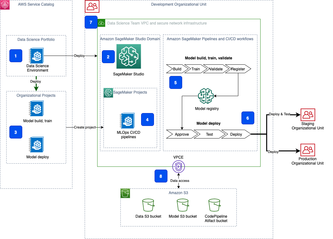
In Part 1 of this series of posts, we offered step-by-step guidance for using Amazon SageMaker, SageMaker projects and Amazon SageMaker Pipelines, and AWS services such as Amazon Virtual Private Cloud (Amazon VPC), AWS CloudFormation, AWS Key Management Service (AWS KMS), and AWS Identity and Access Management (IAM) to implement secure architectures for multi-account enterprise machine learning (ML) environments.

In this second and final part, we provide instructions for deploying the solution from the source code GitHub repository to your account or accounts and experimenting with the delivered SageMaker notebooks.

Solution overview

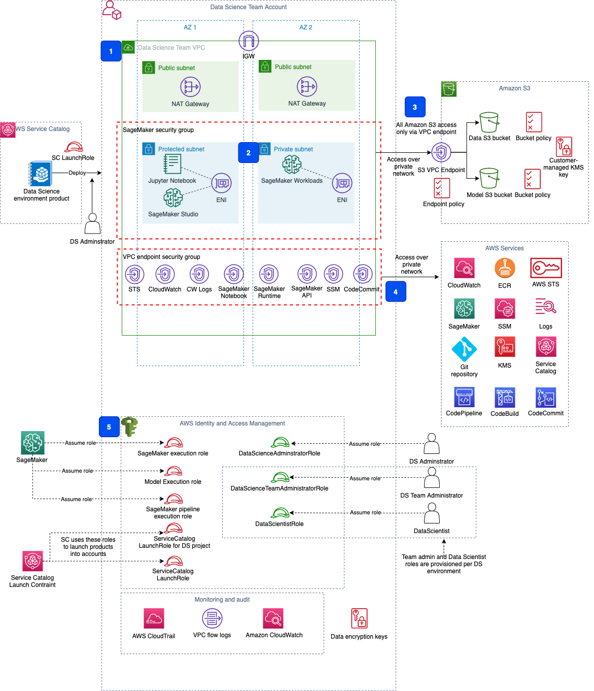
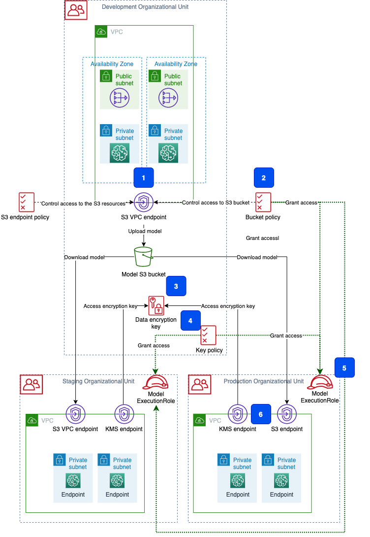
The provided CloudFormation templates provision all the necessary infrastructure and security controls in your account. An Amazon SageMaker Studio domain is also created by the CloudFormation deployment process. The following diagram shows the resources and components that are created in your account.

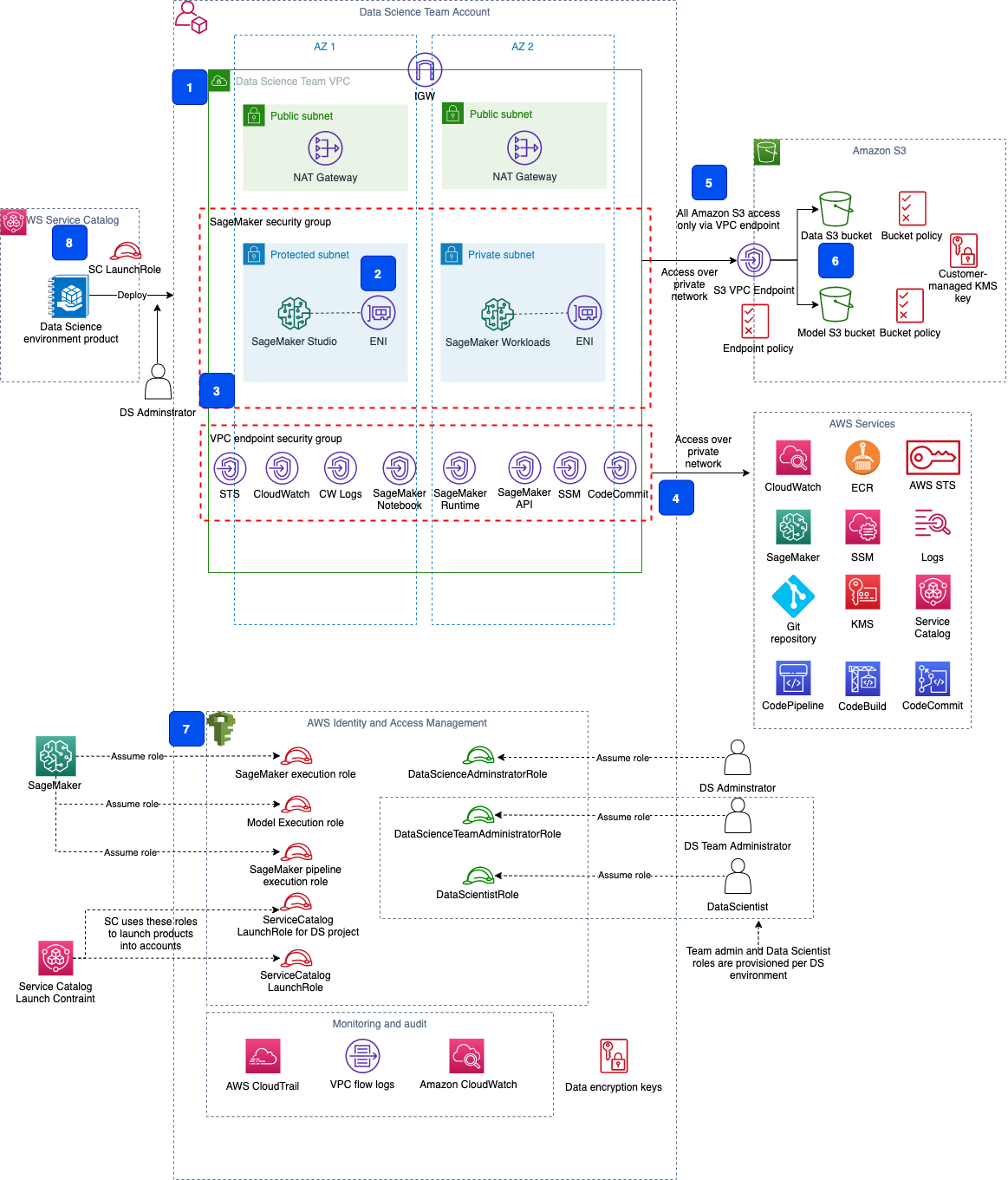
The components are as follows:

1. The network infrastructure with a VPC, route tables, and public and private subnets in each Availability Zone, NAT gateway, and internet gateway.
2. A Studio domain deployed into the VPC, private subnets, and security group. Each elastic network interface used by Studio is created within a private designated subnet and attached to designated security groups.
3. Security controls with two security groups: one for Studio, and one any SageMaker workloads and for VPC endpoints.
4. VPC endpoints to enable a private connection between your VPC and AWS services by using private IP addresses.
5. An S3 VPC endpoint to access your Amazon Simple Storage Service (Amazon S3) buckets via AWS PrivateLink and enable additional access control via an VPC endpoint policy.
6. S3 buckets for storing your data and models. The access to the buckets is controlled by bucket policies. The data in the S3 buckets is encrypted using AWS KMS customer master keys.
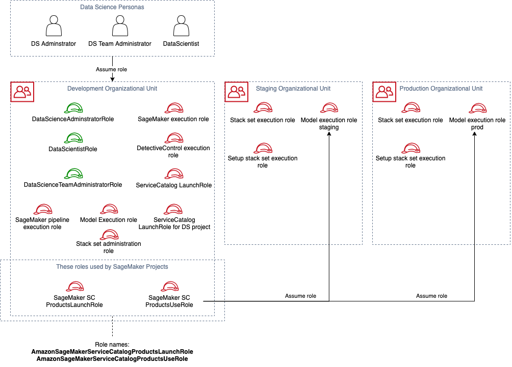
7. A set of AWS Identity and Access Management (IAM) roles for users and services. These roles enable segregation of responsibilities and serve as an additional security control layer.
8. An AWS Service Catalog portfolio, which is used to deploy a data science environment and SageMaker MLOps project templates.

The source code and all AWS CloudFormation templates for the solution and MLOps projects are provided in the GitHub repository.

Prerequisites

To deploy the solution, you must have administrator (or power user) permissions for your AWS account to package the CloudFormation templates, upload templates in an S3 bucket, and run the deployment commands.

If you don’t have the AWS Command Line Interface (AWS CLI), see Installing, updating, and uninstalling the AWS CLI.

Deploy a CloudFormation template to package and upload the solution templates

Before you can deploy the delivered CloudFormation templates with the solution, they must be packaged and uploaded to an S3 bucket for deployment.

First, you deploy a simple CloudFormation template package-cfn.yaml. The template creates an AWS CodeBuild project, which packages and uploads the solution deployment templates into a specified S3 bucket.

To follow along with the deployment instructions, run the following commands in your CLI terminal (all commands have been tested for macOS 10.15.7)

1. Clone the GitHub repository:

   git clone https://github.com/aws-samples/amazon-sagemaker-secure-mlops.git
   cd amazon-sagemaker-secure-mlops

2. If you don’t have an S3 bucket, you must create a new one (skip this step if you already have an S3 bucket):

   S3_BUCKET_NAME=<your new S3 bucket name>
   aws s3 mb s3://${S3_BUCKET_NAME} --region $AWS_DEFAULT_REGION

3. Upload the source code .zip file sagemaker-secure-mlops.zip to the S3 bucket:

   S3_BUCKET_NAME=<your existing or just created S3 bucket name>
   aws s3 cp sagemaker-secure-mlops.zip s3://${S3_BUCKET_NAME}/sagemaker-mlops/

4. Deploy the CloudFormation template:

   STACK_NAME=sagemaker-mlops-package-cfn
   aws cloudformation deploy 
           --template-file package-cfn.yaml 
           --stack-name $STACK_NAME 
           --capabilities CAPABILITY_NAMED_IAM 
           --parameter-overrides 
           S3BucketName=$S3_BUCKET_NAME

5. Wait until deployment is complete and check that the deployment templates are uploaded into the S3 bucket. You may have to wait a few minutes before the templates appear in the S3 bucket:

   aws s3 ls s3://${S3_BUCKET_NAME}/sagemaker-mlops/ --recursive

At this point, all the deployment CloudFormation templates are packaged and uploaded to your S3 bucket. You can proceed with the further deployment steps.

Deployment options

You have a choice of different independent deployment options using the delivered CloudFormation templates:

• Data science environment quickstart – Deploy an end-to-end data science environment with the majority of options set to default values. This deployment type supports a single-account model deployment workflow only. You can change only a few deployment parameters.
• Two-step deployment via AWS CloudFormation – Deploy the core infrastructure in the first step and then deploy a data science environment, both as CloudFormation templates. You can change any deployment parameter.
• Two-step deployment via AWS CloudFormation and AWS Service Catalog – Deploy the core infrastructure in the first step and then deploy a data science environment via AWS Service Catalog. You can change any deployment parameter.

In this post, we use the latter deployment option to demonstrate using AWS Service Catalog product provisioning. To explore and try out other deployment options, refer to the instructions in the README.md.

Multi-account model deployment workflow prerequisites

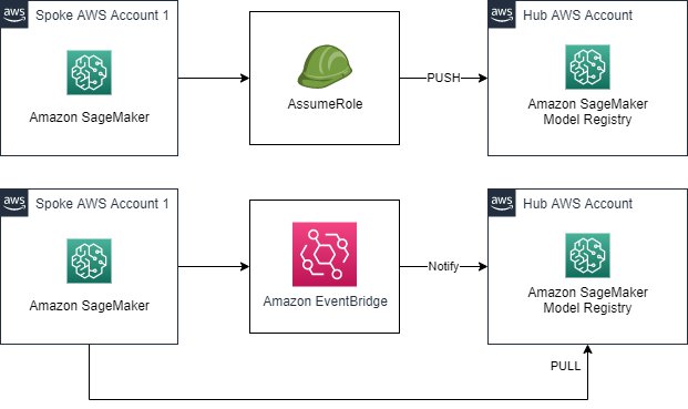
Multi-account model deployment requires VPC infrastructure and specific execution roles to be provisioned in the target accounts. The provisioning of the infrastructure and the roles is done automatically during the deployment of the data science environment as a part of the overall deployment process. To enable a multi-account setup, you must provide the staging and production organizational unit (OU) IDs or the staging and production lists as CloudFormation parameters for the deployment.

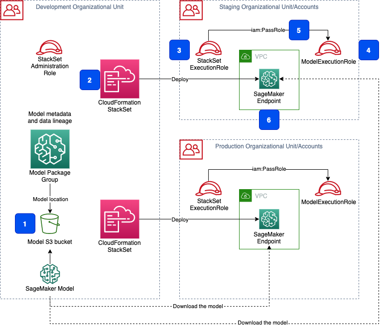
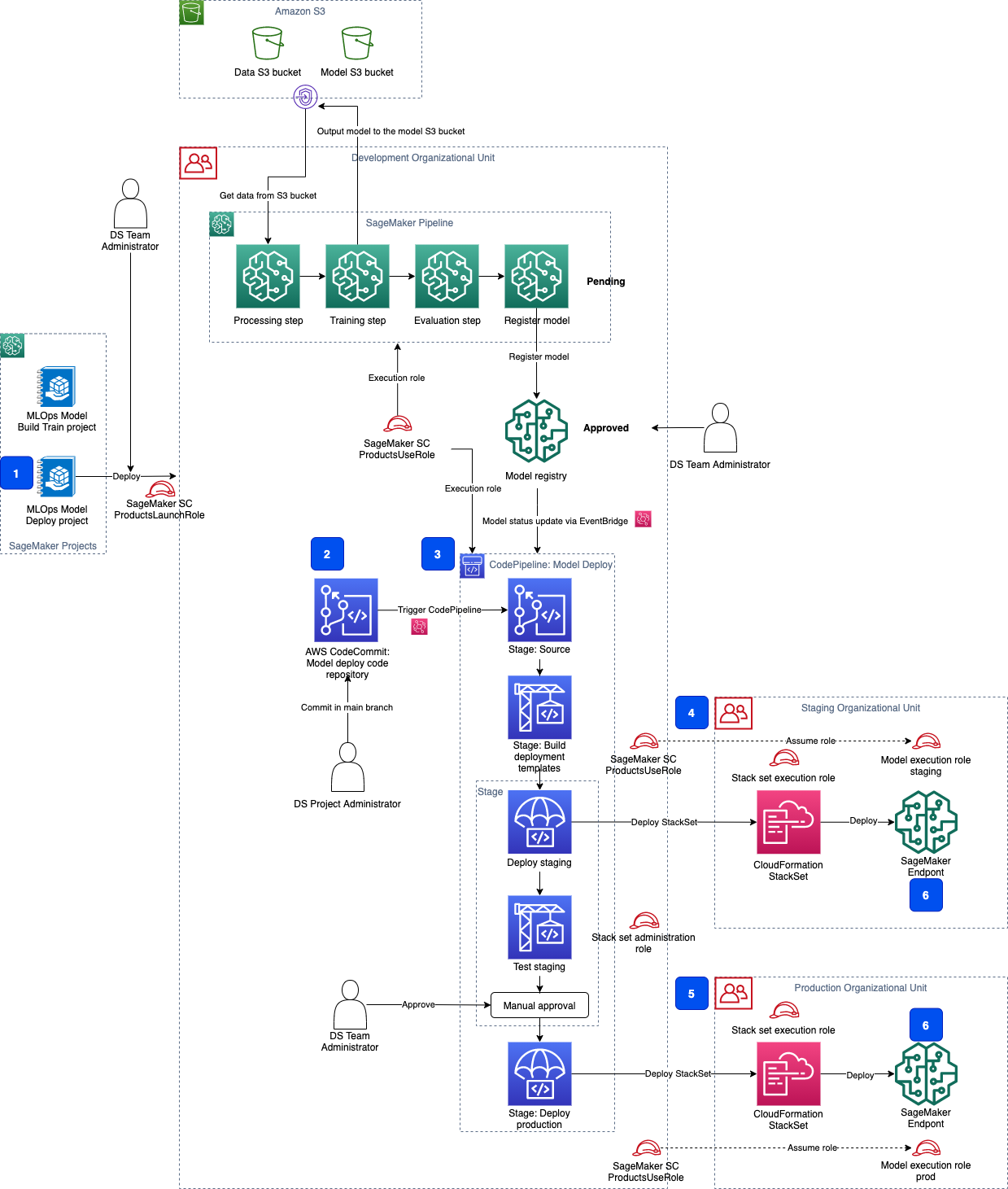
The following diagram shows how we use the CloudFormation stack sets to deploy the required infrastructure to the target accounts.

Two stack sets—one for the VPC infrastructure and another for the IAM roles—are deployed into the target accounts for each environment type: staging and production.

A one-time setup is needed to enable a multi-account model deployment workflow with SageMaker MLOps projects. You don’t need to perform this setup if you’re going to use single-account deployment only.

1. Provision the target account IAM roles
2. Register a delegated administrator for AWS Organizations

Provision the target account IAM roles

Provisioning a data science environment uses a CloudFormation stack set to deploy the IAM roles and VPC infrastructure into the target accounts. The solution uses the SELF_MANAGED stack set permission model and needs two IAM roles:

• AdministratorRole in the development account (main account)
• SetupStackSetExecutionRole in each of the target accounts

The role AdministratorRole is automatically created during the solution deployment. You only need to provision the latter role before starting the deployment. You can use the delivered CloudFormation template env-iam-setup-stacksest-role.yaml or your own process for provision an IAM role. See the following code:

# STEP 1:
# SELF_MANAGED stack set permission model:
# Deploy a stack set execution role to _EACH_ of the target accounts in both staging and prod OUs or account lists
# This stack set execution role is used to deploy the target accounts stack sets in env-main.yaml
# !!!!!!!!!!!! RUN THIS COMMAND IN EACH OF THE TARGET ACCOUNTS !!!!!!!!!!!!
ENV_NAME=sm-mlops
ENV_TYPE=# use your own consistent environment stage names like "staging" and "prod"
STACK_NAME=$ENV_NAME-setup-stackset-role
ADMIN_ACCOUNT_ID=<DATA SCIENCE DEVELOPMENT ACCOUNT ID>
SETUP_STACKSET_ROLE_NAME=$ENV_NAME-setup-stackset-execution-role

# Delete stack if it exists
aws cloudformation delete-stack --stack-name $STACK_NAME

aws cloudformation deploy 
                --template-file cfn_templates/env-iam-setup-stackset-role.yaml 
                --stack-name $STACK_NAME 
                --capabilities CAPABILITY_NAMED_IAM 
                --parameter-overrides 
                EnvName=$ENV_NAME 
                EnvType=$ENV_TYPE 
                StackSetExecutionRoleName=$SETUP_STACKSET_ROLE_NAME 
                AdministratorAccountId=$ADMIN_ACCOUNT_ID

aws cloudformation describe-stacks 
    --stack-name $STACK_NAME 
    --output table 
    --query "Stacks[0].Outputs[*].[OutputKey, OutputValue]"

Note the name of the provisioned IAM role StackSetExecutionRoleName in the stack output. You use this name in the AWS Service Catalog-based deployment as the SetupStackSetExecutionRoleName parameter.

Register a delegated administrator for AWS Organizations

This step is only needed if you want to use an AWS Organizations-based OU setup.

A delegated administrator account must be registered in order to enable the ListAccountsForParent Organizations API call. If the data science account is already the management account in Organizations, you must skip this step. See the following code:

# STEP 2:
# Register a delegated administrator to enable AWS Organizations API permission for non-management account
# Must be run under administrator in the AWS Organizations _management account_
aws organizations register-delegated-administrator 
    --service-principal=member.org.stacksets.cloudformation.amazonaws.com 
    --account-id=$ADMIN_ACCOUNT_ID

aws organizations list-delegated-administrators  
    --service-principal=member.org.stacksets.cloudformation.amazonaws.com

Deployment via AWS CloudFormation and the AWS Service Catalog

This deployment option first deploys the core infrastructure including the AWS Service Catalog portfolio of data science products. In the second step, the data science administrator deploys a data science environment via the AWS Service Catalog.

The deployment process creates all the necessary resources for the data science platform, such as VPC, subnets, NAT gateways, route tables, and IAM roles.

Alternatively, you can select your existing network and IAM resources to be used for stack deployment. In this case, set the corresponding CloudFormation and AWS Service Catalog product parameters to the names and ARNs of your existing resources. You can find the detailed instructions for this use case in the code repository.

Deploy the base infrastructure

In this step, you deploy the shared core infrastructure into your AWS account. The stack (core-main.yaml) provisions the following:

• Shared IAM roles for data science personas and services (optionally, you may provide your own IAM roles)
• An AWS Service Catalog portfolio to provide a self-service deployment for the data science administrator user role

You must delete two pre-defined SageMaker roles – AmazonSageMakerServiceCatalogProductsLaunchRole and AmazonSageMakerServiceCatalogProductsUseRole – if they exist in your AWS account before deploying the base infrastructure.

The following command uses the default values for the deployment options. You can specify additional parameters via ParameterKey=<ParameterKey>, ParameterValue=<Value> pairs in the AWS CloudFormation create-stack call. Set the S3_BUCKET_NAME variable to the name of the S3 bucket where you uploaded the CloudFormation templates:

STACK_NAME="sm-mlops-core"
S3_BUCKET_NAME=<name of the S3 bucket with uploaded solution templates>
aws cloudformation create-stack 
    --template-url https://s3.$AWS_DEFAULT_REGION.amazonaws.com/$S3_BUCKET_NAME/sagemaker-mlops/core-main.yaml 
    --region $AWS_DEFAULT_REGION 
    --stack-name $STACK_NAME  
    --disable-rollback 
    --capabilities CAPABILITY_IAM CAPABILITY_NAMED_IAM 
    --parameters 
        ParameterKey=StackSetName,ParameterValue=$STACK_NAME

After a successful stack deployment, you print out the stack output:

aws cloudformation describe-stacks 
    --stack-name sm-mlops-core  
    --output table 
    --query "Stacks[0].Outputs[*].[OutputKey, OutputValue]"

Deploy a data science environment via AWS Service Catalog

After the base infrastructure is provisioned, the data science administrator user must assume the data science administrator IAM role (AssumeDSAdministratorRole) via the link in the CloudFormation stack output. In this role, users can browse the AWS Service Catalog and then provision a secure Studio environment.

1. First, print the output from the stack deployment:

   aws cloudformation describe-stacks 
       --stack-name sm-mlops-core  
       --output table 
       --query "Stacks[0].Outputs[*].[OutputKey, OutputValue]"

2. Copy and paste the AssumeDSAdministratorRole link to a web browser and switch your role to the data science administrator.
   
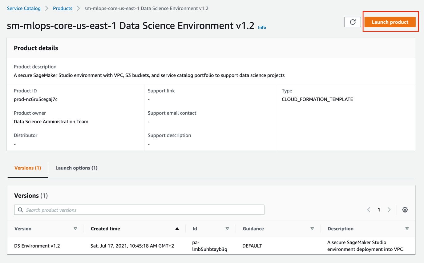
3. On the AWS Service Catalog console, choose Products in the navigation pane.
   

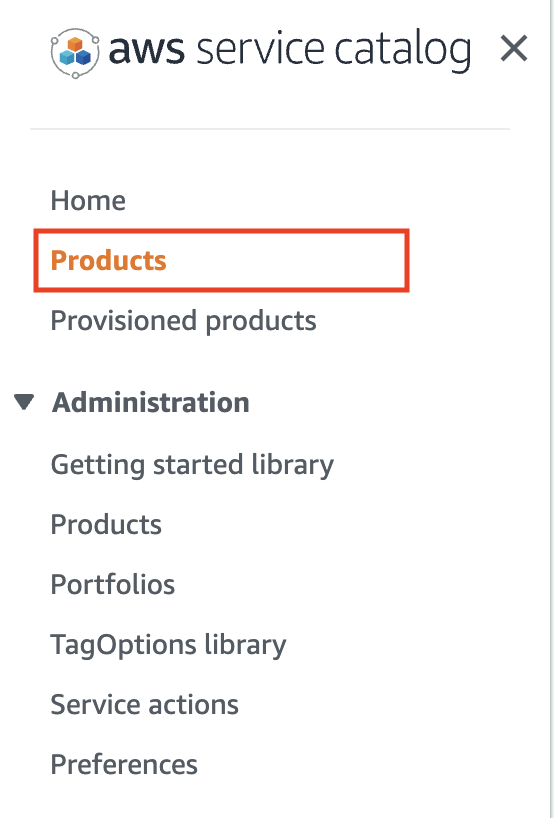
You see the list of the available products for your user role.

4. Choose the product name and then choose Launch product on the product page.
   
5. Fill the product parameters with values specific for your environment.

You provide the values for OU IDs or staging and production account lists and the name for SetupStackSetExecutionRole if you want to enable multi-account model deployment; otherwise keep these parameters empty.

You must provide two required parameters:

• S3 bucket name with MLOps seed code – Use the S3 bucket where you packaged the CloudFormation templates.
  

• Availability Zones – You need at least two Availability Zones for your SageMaker model deployment workflow.
  

Wait until AWS Service Catalog finishes provisioning the data science environment stack and the product status becomes Available. The data science environment provisioning takes about 20 minutes to complete.

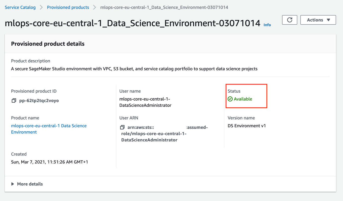
Now you have provisioned the data science environment and can start experimenting with it.

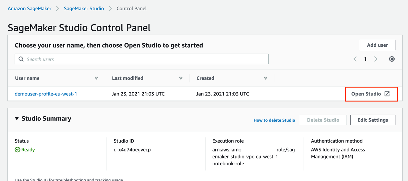
Launch Studio and experiment

To launch Studio, open the SageMaker console, choose Open SageMaker Studio, and choose Open Studio.

You can find some experimentation ideas and step-by-step instructions in the provided GitHub code repository:

• Explore the AWS Service Catalog portfolio
• Test secure access to Amazon S3
• Test preventive IAM policies
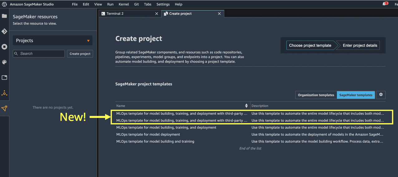
• Provision a new MLOps project
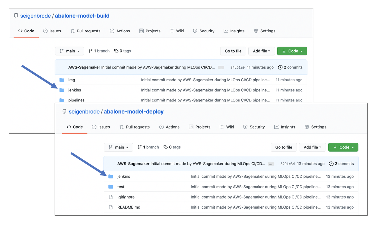
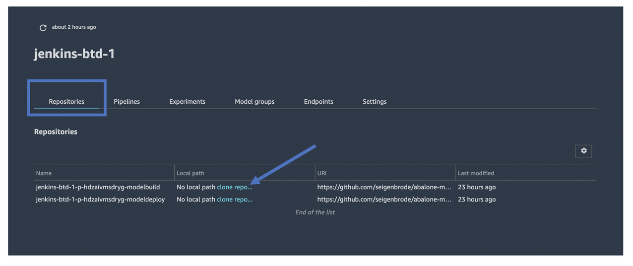
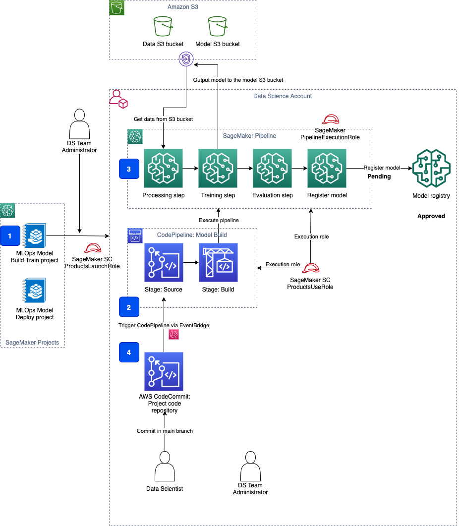
• Work with a model build, train, validate project
• Work with a model deploy project

Reference architectures on AWS

For further research, experimentation, and evaluation, you can look into the reference architectures available on AWS Solutions as vetted ready-to-use AWS MLOps Framework and on AWS Quick Starts as Amazon SageMaker with Guardrails on AWS delivered by one of the AWS Partners.

Clean up

Provisioning a data science environment with Studio, VPC, VPC endpoints, NAT gateways, and other resources creates billable components in your account. If you experiment with any delivered MLOps project templates, it may create additional billable resources such as SageMaker endpoints, inference compute instances, and data in S3 buckets. To avoid charges, you should clean up your account after you have finished experimenting with the solution.

The solution provides a cleanup notebook with a full cleanup script. This is the recommended way to clean up resources. You can also follow the step-by-step instructions in this section.

Clean up after working with MLOps project templates

The following resources should be removed:

• CloudFormation stack sets with model deployment in case you run a model deploy pipeline. Stack set deletion removes provisioned SageMaker endpoints and associated resources from all involved accounts.
• SageMaker projects and corresponding S3 buckets with project and pipeline artifacts.
• Any data in the data and models S3 buckets.

The provided notebooks for MLOps projects—sagemaker-model-deploy and sagemaker-pipelines-project—include cleanup code to remove resources. Run the code cells in the cleanup section of the notebook after you have finished working with the project.

1. Delete the CloudFormation stack sets with the following code:

   import time
   
   cf = boto3.client("cloudformation")
   
   for ss in [
           f"sagemaker-{project_name}-{project_id}-deploy-{env_data['EnvTypeStagingName']}",
           f"sagemaker-{project_name}-{project_id}-deploy-{env_data['EnvTypeProdName']}"
           ]:
       accounts = [a["Account"] for a in cf.list_stack_instances(StackSetName=ss)["Summaries"]]
       print(f"delete stack set instances for {ss} stack set for the accounts {accounts}")
       r = cf.delete_stack_instances(
           StackSetName=ss,
           Accounts=accounts,
           Regions=[boto3.session.Session().region_name],
           RetainStacks=False,
       )
       print(r)
   
       time.sleep(180)
   
       print(f"delete stack set {ss}")
       r = cf.delete_stack_set(
           StackSetName=ss
       )

2. Delete the SageMaker project:

   print(f"Deleting project {project_name}:{sm.delete_project(ProjectName=project_name)}")

3. Remove the project S3 bucket:

   !aws s3 rb s3://sm-mlops-cp-{project_name}-{project_id} --force

Remove the data science environment stack

After you clean up MLOps project resources, you can remove the data science stack.

The AWS CloudFormation delete-stack command doesn’t remove any non-empty S3 buckets. You must empty the data and models from the data science environment S3 buckets before you can delete the data science environment stack.

1. Remove the VPC-only access policy from the data and model bucket in order to be able to delete objects from a CLI terminal:

   ENV_NAME=<use default name ‘sm-mlops’ or your data science environment name you chosen when you created the stack>
   aws s3api delete-bucket-policy --bucket $ENV_NAME-dev-${AWS_DEFAULT_REGION}-data
   aws s3api delete-bucket-policy --bucket $ENV_NAME-dev-${AWS_DEFAULT_REGION}-models

2. Empty the S3 buckets. This is a destructive action. The following command deletes all files in the data and models S3 buckets:

   aws s3 rm s3://$ENV_NAME-dev-$AWS_DEFAULT_REGION-data --recursive
   aws s3 rm s3://$ENV_NAME-dev-$AWS_DEFAULT_REGION-models --recursive

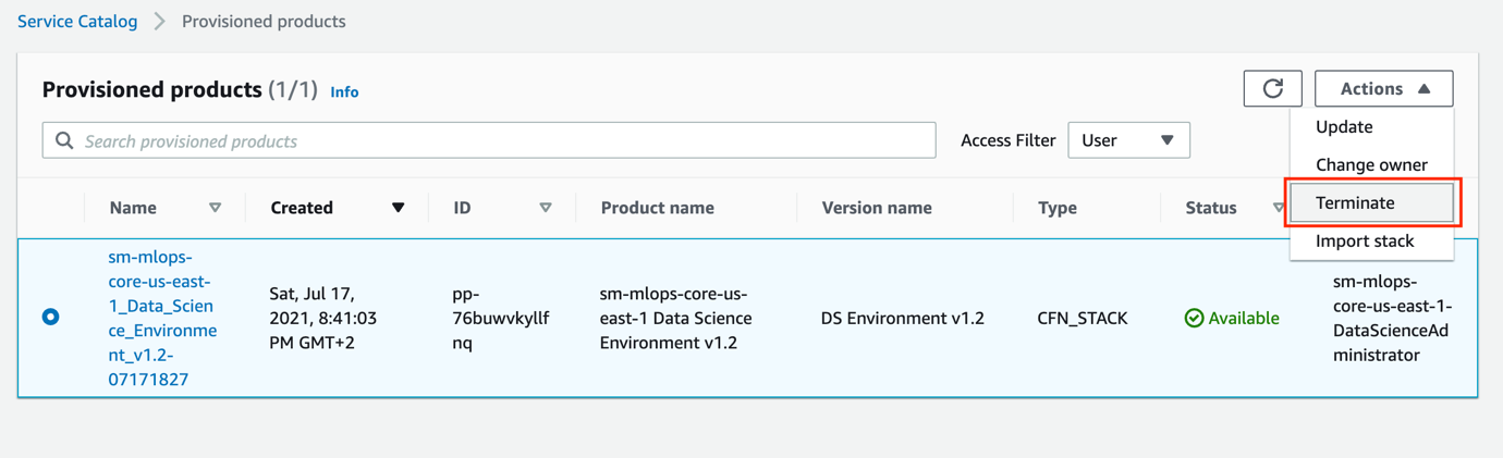
Next, we stop the AWS Service Catalog product.

3. Assume the DSAdministratorRole role via the link in the CloudFormation stack output.
4. On the AWS Service Catalog, on the Provisioned products page, select your product and choose Terminate on the Actions menu.
   
5. Delete the core infrastructure CloudFormation stacks:

aws cloudformation delete-stack --stack-name sm-mlops-core
aws cloudformation wait stack-delete-complete --stack-name sm-mlops-core
aws cloudformation delete-stack --stack-name sagemaker-mlops-package-cfn

Remove the SageMaker domain file system

The deployment of Studio creates a new Amazon Elastic File System (Amazon EFS) file system in your account. This file system is shared with all users of Studio and contains home directories for Studio users and may contain your data.

When you delete the data science environment stack, the Studio domain, user profile, and apps are also deleted. However, the file system isn’t deleted, and is kept as is in your account. Additional resources are created by Studio and retained upon deletion together with the file system:

• Amazon EFS mounting points in each private subnet of your VPC
• An elastic network interface for each mounting point
• Security groups for Amazon EFS inbound and outbound traffic

To delete the file system and any Amazon EFS-related resources in your AWS account created by the deployment of this solution, perform the following steps after running the delete-stack commands (from the preceding step).

This is a destructive action. All data on the file system will be deleted (SageMaker home directories). You may want to back up the file system before deletion.

6. On the Amazon EFS console, choose the SageMaker file system.
7. On the Tags tab, locate the tag key ManagedByAmazonSageMakerResource. Its tab value contains the SageMaker domain ID.
   
8. Choose Delete to delete the file system.
9. On the Amazon VPC console, delete the data science environment VPC.

Alternatively, you can remove the file using the following AWS CLI commands. First, list the SageMaker domain IDs for all file systems with the SageMaker tag:

aws efs describe-file-systems 
  --query 'FileSystems[].Tags[?Key==`ManagedByAmazonSageMakerResource`].Value[]'

Then copy the SageMaker domain ID and run the following script from the solution directory:

SM_DOMAIN_ID=#SageMaker domain id
pipenv run python3 functions/pipeline/clean-up-efs-cli.py $SM_DOMAIN_ID

Conclusion

In this series of posts, we presented the main functional and infrastructure components, implementation guidance, and source code for an end-to-end enterprise-grade ML environment. This solution implements a secure development environment with multi-layer security controls, CI/CD MLOps automation pipelines, and the deployment of the production inference endpoints for model serving.

You can use the best practices, architectural solutions, and code samples to design and build your own secure ML environment. If you have any questions, please reach out to us in the comments!

About the Author

Yevgeniy Ilyin is a Solutions Architect at AWS. He has over 20 years of experience working at all levels of software development and solutions architecture and has used programming languages from COBOL and Assembler to .NET, Java, and Python. He develops and codes cloud native solutions with a focus on big data, analytics, and data engineering.

Read More

Amazon SageMaker Studio is a web-based, integrated development environment (IDE) for machine learning (ML) that lets you build, train, debug, deploy, and monitor your ML models.

Although Studio provides all the tools you need to take your models from experimentation to production, you need a robust and secure model deployment process. This process must fulfill your organization’s operational and security requirements.

Amazon SageMaker and Studio provide a wide range of specialized functionality for building highly secure, scalable, and flexible MLOps platforms to cover your model deployment use cases and requirements. Three SageMaker services, SageMaker Pipelines, SageMaker Projects, and SageMaker Model Registry, build a foundation to implement enterprise-grade secure multi-account model deployment workflow.

In combination with other AWS services, such as Amazon Virtual Private Cloud (Amazon VPC), AWS CloudFormation, and AWS Identity and Access Management (IAM), SageMaker MLOps can deliver solutions for the most demanding security and governance requirements.

Using a multi-account data science environment to meet security, reliability, and operational needs is a good DevOps practice. A multi-account strategy is paramount to achieve strong workload and data isolation, support multiple unrelated teams and projects, ensure fine-grained security and compliance control, facilitate billing, and create cost transparency.

In this two-part post, we offer guidance for using AWS services and SageMaker functionalities, and recommend practices for implementing a production-grade ML platform and secure, automated, multi-account model deployment workflows.

Such ML platforms and workflows can fulfill stringent security requirements, even for regulated industries such as financial services. For example, customers in regulated industries often don’t allow any internet access in ML environments. They often use only VPC endpoints for AWS services. They implement end-to-end data encryption in transit and at rest, and enforce workload isolation for individual teams in a line of business in multi-account organizational structures.

Part 1 of this series focuses on providing a solution architecture overview, in which we explain the security controls employed and how they are implemented. We also look at MLOps automation workflows with SageMaker projects and Pipelines.

In Part 2, we walk through deploying the solution with hands-on SageMaker notebooks.

Solution overview

The post Multi-account model deployment with Amazon SageMaker Pipelines shows a conceptual setup of a multi-account MLOps environment based on Pipelines and SageMaker projects.

The solution presented in this post is built for an actual use case for an AWS customer in the financial services industry. It focuses on the security, automation, and governance aspects of multi-account ML environments. It provides a fully automated provisioning of Studio into your private VPC, subnets and security groups using CloudFormation templates, and stack sets. Compared to the previous post, this solution implements network traffic and access controls with VPC endpoints, security groups, and fine-grained permissions with designated IAM roles. To reflect the real-life ML environment requirements, the solution enforces end-to-end data encryption at rest and in transit.

The following diagram shows the overview of the solution architecture and the deployed components.

Let’s look at each group of components in more detail.

Component 1: AWS Service Catalog

The end-to-end deployment of the data science environment is delivered as an AWS Service Catalog self-provisioned product. One of the main advantages of using AWS Service Catalog for self-provisioning is that authorized users can configure and deploy available products and AWS resources on their own, without needing full privileges or access to AWS services. The deployment of all AWS Service Catalog products happens under a specified service role with the defined set of permissions, which are unrelated to the user’s permissions.

Component 2: Studio domain

The Data Science Environment product in the AWS Service Catalog creates a Studio domain. A Studio domain consists of a list of authorized users, configuration settings, and an Amazon Elastic File System (Amazon EFS) volume. The Amazon EFS volume contains data for the users, including notebooks, resources, and artifacts.

Components 3 and 4: SageMaker MLOps project templates

The solution delivers the customized versions of SageMaker MLOps project templates. Each MLOps template provides an automated model building and deployment pipeline using continuous integration and continuous delivery (CI/CD). The delivered templates are configured for the secure multi-account model deployment and are fully integrated in the provisioned data science environment. The project templates are provisioned in Studio via AWS Service Catalog. The templates include the seed code repository with Studio notebooks, which implements a secure setup of SageMaker workloads such as processing, training jobs, and pipelines.

Components 5 and 6: CI/CD workflows

The MLOps projects implement CI/CD using Pipelines and AWS CodePipeline, AWS CodeCommit, and AWS CodeBuild. SageMaker project templates also support a CI/CD workflow using Jenkins and GitHub as the source repository.

Pipelines is responsible for orchestrating workflows across each step of the ML process and task automation, including data loading, data transformation, training, tuning and validation, and deployment. Each model is tracked via SageMaker Model Registry, which stores the model metadata, such as training and validation metrics and data lineage, and retains model versions and the approval status of the model.

CodePipeline deploys the model to the designated target accounts with staging and production environments. The necessary resources are pre-created by CloudFormation templates during infrastructure creation.

This solution supports secure multi-account model deployment using AWS Organizations or via simple target account lists.

Component 7: Secure infrastructure

The Studio domain is deployed in a dedicated VPC. Each elastic network interface used by a SageMaker domain or workload is created within a private dedicated subnet and attached to the specified security groups. The data science environment VPC can be configured with internet access via an optional NAT gateway. You can also run this VPC in internet-free mode without any inbound or outbound internet access.

All access to the AWS public services is routed via AWS PrivateLink. Traffic between your VPC and the AWS services doesn’t leave the Amazon network and isn’t exposed to the public internet.

Component 8: Data security

All data in the data science environment, which is stored in Amazon Simple Storage Service (Amazon S3) buckets and Amazon Elastic Block Store (Amazon EBS) and EFS volumes, is encrypted at rest using customer managed CMKs. All data transfer between platform components, API calls, and inter-container communication is protected using the Transport Layer Security (TLS 1.2) protocol.

Data access from the Studio notebooks or any SageMaker workload to the environment’s S3 buckets is governed by the combination of the S3 bucket and user policies and S3 VPC endpoint policy.

Multi-account structure

With the goal of illustrating best practices, this solution implements the following three account groups:

• Development – This account is used by data scientists and ML engineers to perform experimentation and development. Data science tools such as Studio are used in the development account. S3 buckets with data and models, code repositories, and CI/CD pipelines are hosted in this account. Models are built, trained, validated, and registered in the model repository in this account.
• Testing/staging/UAT – Validated and approved models are first deployed to the staging account, where the automated unit and integration tests are run. Data scientists and ML engineers have read-only access to this account.
• Production – Fully tested and approved models from the staging accounts are deployed to the production account for both online and batch inference.

Depending on your specific security and governance requirements and your development organization, for the production setup, we recommend using two additional account groups:

• Shared services – This account hosts common resources like team code repositories, CI/CD pipelines for MLOps workflows, Docker image repositories, service catalog portfolios, model registries, and library package repositories.
• Data management – A dedicated AWS account to store and manage all data for the ML process. We recommend implementing strong data security and governance practices using AWS Data Lake and AWS Lake Formation.

Each of these account groups can have multiple AWS accounts and environments for developing and testing services and storing different types of data.

Environment layers

In the following sections, we look at the whole data science environment in terms of layers:

• Network and security infrastructure
• IAM roles and cross-account permission setup
• Application stack consisting of Studio and SageMaker MLOps projects

In Part 2 of this post, you deploy the solution into your AWS account for further experimentation.

Secure infrastructure

We use AWS foundational services such as VPC, security groups, subnets, and NAT gateways to create the secure infrastructure for the data science environment. The following diagram shows the deployment architecture for the solution.

VPC, subnets, routes, and internet access

Our Studio domain is deployed into a dedicated data science VPC using VPC Only mode (Step 1 in the preceding architecture). In this mode, you use your own control flow for the internet traffic, like a NAT gateway or AWS Network Firewall. You can also create an internet-free VPC for your highly secure workloads. Any SageMaker workload launched in the VPC creates an elastic network interface in the specified subnet. You can apply all available layers of security controls—security groups, network ACLs, VPC endpoints, AWS PrivateLink, or Network Firewall endpoints—to the internal network and internet traffic to exercise fine-grained control of network access in Studio. For a detailed description of network configurations and security controls, refer to Securing Amazon SageMaker Studio connectivity using a private VPC. If you must control ingress and egress network traffic or apply any filtering rules, you can use Network Firewall as described in Securing Amazon SageMaker Studio internet traffic using AWS Network Firewall.

All SageMaker workloads, like Studio notebooks, processing or training jobs, and inference endpoints, are placed in the private subnets within the dedicated security group (2). This security group doesn’t allow any ingress from any network interface outside the group except for intra-group communications.

VPC endpoints

All access to Amazon S3 is routed via the gateway-type S3 VPC endpoint (3). You control access to the resources behind a VPC endpoint with a VPC endpoint policy. The combination of the VPC endpoint policy and the S3 bucket policy ensures that only specified buckets can be accessed, and these buckets can be accessed only via the designated VPC endpoints. The solution provisions two buckets: Data and Models. You can extend the CloudFormation templates to accommodate your data storage requirements, create additional S3 buckets, or tighten the data access permissions.

Studio and Studio notebooks communicate with various AWS services, such as the SageMaker backend and APIs, Amazon SageMaker Runtime, AWS Security Token Service (AWS STS), Amazon CloudWatch, AWS Key Management Service (AWS KMS), and others.

The solution uses a private connection over interface-type VPC endpoints (4) to access these AWS services. All VPC endpoints are placed in the dedicated security group to control the inbound and outbound network access. You can find a list with the recommended VPC endpoints to be set up for Studio in the following AWS technical guide.

IAM roles and preventive security controls

The solution uses IAM to set up personas and service execution roles (5). You can assign fine-grained permissions policies on the least privilege principle to various SageMaker execution roles, used to run different workloads, such as processing or training jobs, pipelines, or inference. You can implement preventive security controls using SageMaker-specific IAM condition keys. For example, the solution enforces usage of VPC isolation with private subnets and usage of the security groups for SageMaker notebook instances, processing, training, and tuning jobs, as well as for models for the SageMaker execution role:

{
    "Action": [
        "sagemaker:CreateNotebookInstance",
        "sagemaker:CreateHyperParameterTuningJob",
        "sagemaker:CreateProcessingJob",
        "sagemaker:CreateTrainingJob",
        "sagemaker:CreateModel"
    ],
    "Resource": "*",
    "Effect": "Deny",
    "Condition": {
        "Null": {
            "sagemaker:VpcSubnets": "true",
	    "sagemaker:VpcSecurityGroupIds": "true"
        }
    }
}

For a detailed discussion of the security controls and best practices, refer to Building secure machine learning environments with Amazon SageMaker.

Cross-account permission and infrastructure setup

When using a multi-account setup for your data science platform, you must focus on setting up and configuring IAM roles, resource policies, and cross-account trust and permissions polices with special attention to the following topics:

• How do you set up access to the resources in one account from authorized and authenticated roles and users from another accounts?
• What roles in one (target) account must be assumed by a role in another (source) account to perform a specific action in the target account?
• Does the assumed role in the target account have a trust policy for a role in the source account, and does the role in the source account have iam:AssumeRole permission in its permissions policy for the principal in the target account? For more information, see How to use trust policies with IAM roles.
• Do your AWS CloudFormation deployment roles have iam:PassRole permission for the execution roles they assign to the created resources?
• How do you configure access control and resource isolation for teams or groups within Studio? For an overview and recipes for the implementation, see Configuring Amazon SageMaker Studio for teams and groups with complete resource isolation.

The solution implements the following IAM roles in its multi-account setup, as shown in the diagram.

User persona IAM roles and various execution roles are created in the development account as we run Studio and perform development work there. We must create the following IAM roles in the staging and production accounts:

• Stack set execution roles – Used to deploy various resources into target accounts during the initial environment provision and for multi-account CI/CD MLOps workflows
• Model execution roles – Assumed by SageMaker to access model artifacts and the Docker image for deployment on ML compute instances (SageMaker inference)

These roles are assumed by the roles in the development account.

Configure permissions for multi-account model deployment

In this section, we look closer at the permission setup for multi-account model deployment.

First, we must understand how the multi-account CI/CD model pipeline deploys the model to SageMaker endpoints in the target accounts. The following diagram shows the model deployment process.

After model training and validation, the model is registered in the model registry. The model registry stores the model metadata, and all model artifacts are stored in an S3 bucket (Step 1 in the preceding diagram). The CI/CD pipeline uses CloudFormation stack sets (2) to deploy the model in the target accounts. The CloudFormation service assumes the role StackSetExecutionRole (3) in the target account to perform the deployment. SageMaker also assumes the role ModelExecutionRole (4) to access the model metadata and download the model artifacts from the S3 bucket. The StackSetExecutionRole role must have iam:PassRole permission (5) for ModelExecutionRole to be able to pass the role successfully at stack provisioning time. Finally, the model is deployed to a SageMaker endpoint (6).

For a successful deployment, ModelExecutionRole needs access to the model, which is saved in an S3 bucket, and to the corresponding AWS KMS encryption keys in the development account, because the data in the S3 bucket is encrypted.

Both the S3 bucket and AWS KMS key resource policies have an explicit deny statement if any access request doesn’t arrive via a designated VPC endpoint (following is AWS KMS key policy example):

        - Sid: DenyNoVPC
            Effect: Deny
            Principal: '*'
            Action:
              - kms:Encrypt
              - kms:Decrypt
              - kms:ReEncrypt*
              - kms:GenerateDataKey*
              - kms:DescribeKey
            Resource: '*'
            Condition:
              StringNotEquals:
                'aws:sourceVpce': !Ref VPCEndpointKMSId

To access the S3 bucket and AWS KMS key with ModelExecutionRole, the following conditions must be met:

• ModelExecutionRole must have permissions to access the S3 bucket and AWS KMS key in the development account
• Both S3 bucket and AWS KMS key policies must allow cross-account access from ModelExecutionRole in the corresponding target account
• The S3 bucket and AWS KMS key must be accessed only via a designated VPC endpoint in the target account
• The VPC endpoint ID must be explicitly allowed in both S3 bucket and AWS KMS key policies in the Condition statement

The following diagram shows the infrastructure and IAM configuration for a development, staging, and production account that fulfills these requirements.

All access to the model artifacts is made via the S3 VPC endpoint (Step 1 in the preceding architecture). This VPC endpoint allows access to the model and data in your S3 buckets. The bucket policy (2) for the bucket where the models are stored grants access to the ModelExecutionRole principals (5) in each of the target accounts:

"Sid": "AllowCrossAccount",
"Effect": "Allow",
"Principal": {
    "AWS": [
            "arn:aws:iam::<staging-account>:role/SageMakerModelExecutionRole",
            "arn:aws:iam::<prod-account>:role/SageMakerModelExecutionRole",
            "arn:aws:iam::<dev-account>:root"
        ]
}

We apply the same setup for the data encryption key (3), whose policy (4) grants access to the principals in the target accounts.

SageMaker model-hosting endpoints are placed in the VPC (6) in each of the target accounts. Any access to S3 buckets and AWS KMS keys is made via the corresponding VPC endpoints. The IDs of these VPC endpoints are added to the Condition statement of the bucket and the AWS KMS key’s resource policies:

"Sid": "DenyNoVPC",
"Effect": "Deny",
"Principal": "*",
"Action": [
    "s3:GetObject",
    "s3:PutObject",
    "s3:ListBucket",
    "s3:GetBucketAcl",
    "s3:GetObjectAcl",
    "s3:PutBucketAcl",
    "s3:PutObjectAcl"
    ],
    "Resource": [
        "arn:aws:s3:::sm-mlops-dev-us-east-1-models/*",
        "arn:aws:s3:::sm-mlops-dev-us-east-1-models"
    ],
    "Condition": {
         "StringNotEquals": {
              "aws:sourceVpce": [
                   "vpce-0b82e29a828790da2",
                   "vpce-07ef65869ca950e14",
                   "vpce-03d9ed0a1ba396ff5"
                    ]
         }
    }

SageMaker MLOps projects: Automation pipelines

This solution delivers two MLOps projects as SageMaker project templates:

• Model build, train, and validate pipeline
• Multi-account model deploy pipeline

These projects are fully functional examples that are integrated with the solution infrastructure and multi-layer security controls such as VPC, subnets, security groups, AWS account boundaries, and the dedicated IAM execution roles.

You can find a detailed description of the SageMaker MLOps projects in Building, automating, managing, and scaling ML workflows using Amazon SageMaker Pipelines.

MLOps project template to build, train, validate model

This project is based on the SageMaker project template but has been adapted for this particular solution infrastructure and security controls. The following diagram shows the functional setup of the CI/CD pipeline.

The project creates the following resources comprising the MLOps pipeline:

1. An MLOps template, made available through SageMaker projects and provided via an AWS Service Catalog portfolio.
2. A CodePipeline pipeline with two stages: Source to get the source code of the ML pipeline, and Build to build and run the pipeline.
3. A pipeline to implement a repeatable DAG workflow with individual steps for processing, training, validation, and model registration.
4. A seed code repository in CodeCommit.

The seed code repository contains code to create a multi-step model building pipeline that includes data processing, model training, model evaluation, and conditional model registration (depending on model accuracy) steps. The pipeline implementation in the pipeline.py file trains a linear regression model using the XGBoost algorithm on the well-known UCI Abalone dataset. This repository also includes a build specification file, used by CodePipeline and CodeBuild to run the pipeline automatically.

MLOps project template for multi-account model deployment

This project is based on the SageMaker MLOps template for model deployment, but implements secure multi-account deployment from SageMaker Model Registry to SageMaker hosted endpoints for real-time inference in the staging and production accounts.

The following diagram shows the functional components of the project.

The components are as follows:

1. The MLOps project template, which is deployable as a SageMaker project in Studio.
2. A CodeCommit repository with seed code.
3. The model deployment multi-stage CI/CD CodePipeline pipeline.
4. A staging AWS account or accounts where the model is deployed and tested.
5. A production AWS account or accounts where the model is deployed for production serving.
6. SageMaker endpoints with the approved model hosted in your private VPC.

You can use the delivered seed code to implement your own customized model deployment pipelines with additional tests or approval steps.

Multi-account ML development best practices

In addition to the already discussed MLOps approaches, security controls, and infrastructure setup, the following resources provide a detailed description and overview of the ML development and deployment best practices:

• Build a Secure Enterprise Machine Learning Platform on AWS – Gives a fundamental overview of all parts of an enterprise ML platform
• Building secure machine learning environments with Amazon SageMaker – Delivers a hands-on workshop on building secure environments, and you can use the associated code on GitHub.
• Setting up secure, well-governed machine learning environments on AWS – Describes a common operational model and organizational unit setup patterns for creating secure ML platforms.

Conclusion

In this post, we presented the main building blocks and patterns for implementing a multi-account, secure, and governed ML environment. In Part 2 of this series, you deploy the solution from the source code GitHub repository into your account and experiment with the hands-on SageMaker notebooks.

About the Author

Yevgeniy Ilyin is a Solutions Architect at AWS. He has over 20 years of experience working at all levels of software development and solutions architecture and has used programming languages from COBOL and Assembler to .NET, Java, and Python. He develops and codes cloud native solutions with a focus on big data, analytics, and data engineering.

Read More

Amazon Personalize now enables you to optimize personalized recommendations for a business metric of your choice, in addition to improving relevance of recommendations for your users. You can define a business metric such as revenue, profit margin, video watch time, or any other numerical attribute of your item catalog to optimize your recommendations. Amazon Personalize automatically learns what is relevant to your users, considers the business metric you’ve defined, and recommends the products or content to your users that benefit your overall business goals. Configuring an additional objective is easy. You select any numerical column in your catalog when creating a new solution in Amazon Personalize via the AWS Management Console or the API, and you’re ready to go.

Amazon Personalize enables you to easily add real-time personalized recommendations to your applications without requiring any ML expertise. With Amazon Personalize, you pay for what you use, with no minimum fees or upfront commitments. You can get started with a simple three-step process, which takes only a few clicks on the console or a few simple API calls. First, point Amazon Personalize to your user data, catalog data, and activity stream of views, clicks, purchases, and so on, in Amazon Simple Storage Service (Amazon S3) or upload using an API call. Second, either via the console or an API call, train a custom, private recommendation model for your data (CreateSolution). Third, retrieve personalized recommendations for any user by creating a campaign and using the GetRecommendations API.

The rest of this post walks you through the suggested best practices for generating recommendations for your business in greater detail.

Streaming movie service use case

In this post, we propose a fictitious streaming movie service, and as part of the service we provide movie recommendations using movie reviews from the MovieLens database. We assume the streaming service’s agreement with content providers requires royalties every time a movie is viewed. For our use case, we assume movies that have royalties that range from $0.00 to $0.10 per title. All things being equal, the streaming service wants to provide recommendations for titles that the subscriber will enjoy, but minimize costs by recommending titles with lower royalty fees.

It’s important to understand that a trade-off is made when including a business objective in recommendations. Placing too much weight on the objective can lead to a loss of opportunities with customers as the recommendations presented become less relevant to user interests. If the objective weight doesn’t impart enough impact on recommendations, the recommendations will still be relevant but may not drive the business outcomes you aim to achieve. By testing the models in real-world environments, you can collect data on the impact the objective has on your results and balance the relevance of the recommendations with your business objective.

Movie dataset

The items dataset from MovieLens has a structure as follows.

Amazon Personalize objective optimization requires a numerical field to be defined in the item metadata, which is used when considering your business objective. Because Amazon Personalize optimizes for the largest value in the business metric column, simply passing in the royalty amount results in the recommendations driving customers to those movies with the highest royalties. To minimize royalties, we multiply the royalty field by -1, and capture how much the streaming service will spend in royalties to stream the movie.

In this example, the royalty value ranges from -0.12 to 0. The objective’s value can be an integer or a floating point, and the lowest value is adjusted to zero internally by the service when creating a solution regardless of whether the lowest value is positive or negative. The highest value is adjusted to 1, and other values are interpolated between 0–1, preserving the relative difference between all data points.

For movie recommendations, we use the following schema for the items dataset:

{
    "type": "record",
    "name": "Items",
    "namespace": "com.amazonaws.personalize.schema",
    "fields": [
        {
            "name": "ITEM_ID",
            "type": "string"
        },
        {
            "name": "ROYALTY",
            "type": "float"
        },
        {
            "name": "GENRE",
            "type": [
                "null",
                "string"
              ],
            "categorical": True
        }
    ],
    "version": "1.0"
}

The items dataset includes the mandatory ITEM_ID field, list of genres, and savings fields.

Comparing three solutions

The following diagram illustrates the architecture we use to test the benefits of objective optimization. In this scenario, we use two buckets – Items contains movie data and Interactions contains positive movie reviews. The data from the buckets is loaded into the Amazon Personalize dataset group. Once loaded, three solutions are driven from the two datasets: one solution with objective sensitivity off, a second solution with objective sensitivity set to low, and the third has the objective sensitivity set to high. Each of these solutions drives a corresponding campaign.

After the datasets are loaded in an Amazon Personalize dataset group, we create three solutions to demonstrate the impact of the varied objective optimizations on recommendations. The optimization objective selected when creating an Amazon Personalize solution and can have a sensitivity level set to one of four values: OFF, LOW, MEDIUM, or HIGH. This provides a setting on how much weight to give to the business objective, and in this post we show the impact that these settings can have on recommendation performance. While developing your own models, you should experiment with the sensitivity setting to evaluate what drives the best results for your recommendations. Because the objective optimization maximizes for the business metric, we must select ROYALTY as the objective optimization column.

The following example Python code creates an Amazon Personalize solution:

create_solution_response = personalize.create_solution(
        name = "solution name",
        datasetGroupArn = dataset_group_arn,
        recipeArn = recipe_arn,
        solutionConfig = {
            "optimizationObjective": {
                "itemAttribute": "ROYALTY",
                "objectiveSensitivity":"HIGH"
            }
        }
    )

After the solution versions have been trained, you can compare the offline metrics by calling the DescribeSolutionVersion API or visiting the Amazon Personalize console for each solution version.

In the preceding table, larger numbers are better. For coverage, this is the ratio of items that are present in recommendations compared to the total number of items in the dataset (how many items in your catalog are covered by the recommendation generated). To make sure Amazon Personalize recommends a larger portion of your movie catalog, use a model with a higher coverage score.

The average rewards-at-k metric indicates how the solution version performs in achieving your objective. Amazon Personalize calculates this metric by dividing the total rewards generated by interactions (for example, total revenue from clicks) by the total possible rewards from recommendations. The higher the score, the more gains on average per user you can expect from recommendations.

The mean reciprocal rank (MRR) metric measures the relevance of the highest ranked item in the list, and is important for situations where the user is very likely to select the first item recommended. Normalized discounted cumulative gain at k (NDCG-k) measures the relevance of the highest k items, providing the highest weight to the first k in the list. NDCG is useful for measuring effectiveness when multiple recommendations are presented to users, but highest-rated recommendations are more important than lower-rated recommendations. The Precision-k metric measures the number of relevant recommendations in the top k recommendations.

As the solution weighs the objective higher, metrics tend to show lower relevance for users because the model is selecting recommendations based on user behavior data and the business objective. Amazon Personalize provides the ability to control how much influence the objective imparts on recommendations. If the objective provides too much influence, you can expect it to create a poor customer experience because the recommendations stop being relevant to the user. By running an A/B test, you can collect the data needed to deliver the results that best balance relevance and your business objective.

We can retrieve recommendations from the solution versions by creating an Amazon Personalize campaign for each one. A campaign is a deployed solution version (trained model) with provisioned dedicated capacity for creating real-time recommendations for your users. Because the three campaigns share the same item and interaction data, the only variable in the model is the objective optimization settings. When you compare the recommendations for a randomly selected user, you can see how recommendations can change with varied objective sensitivities.

The following chart shows the results of the three campaigns. The rank indicates the order of relevance that Amazon Personalize has generated for each title for the sample user. The title, year, and royalty amount are listed in each cell. Notice how “The Big Squeeze (1994)” moves to the top of the list from fourth position when objective optimization is turned off. Meanwhile, “The Machine (1994)” drops from first position to fifth position when objective optimization is set to low, and down to 24th position when objective optimization is set to high.

The trend of lower royalties as the objective optimization setting is increased from low to high, as you would expect. The sum of all the royalties for the 25 recommended titles also decreased from $0.59 with no objective optimization to $0.20 with objective optimization set to high.

Conclusion

You can use Amazon Personalize to combine user interaction data with a business objective, thereby improving the business outcomes that recommendations deliver for your business. As we’ve shown, objective optimization influenced the recommendations to lower the costs for the movies in our fictitious movie recommendation service. The trade-off between recommendation relevance and the objective is an important consideration, because optimizing for revenue can make your recommendations less relevant for your users. Other examples include steering users to premium content, promoted content, or items with the highest reviews. This additional objective can improve the quality of the recommendations as well as take into account factors you know are important to your business.

The source code for this post is available on GitHub.

To learn more about Amazon Personalize, visit the product page.

About the Authors

Mike Gillespie is a solutions architect at Amazon Web Services. He works with the AWS customers to provide guidance and technical assistance helping them improve the value of their solutions when using AWS. Mike specializes in helping customers with serverless, containerized, and machine learning applications. Outside of work, Mike enjoys being outdoors running and paddling, listening to podcasts, and photography.

Matt Chwastek is a Senior Product Manager for Amazon Personalize. He focuses on delivering products that make it easier to build and use machine learning solutions. In his spare time, he enjoys reading and photography.

Ge Liu is an Applied Scientist at AWS AI Labs working on developing next generation recommender system for Amazon Personalize. Her research interests include Recommender System, Deep Learning, and Reinforcement Learning.

Abhishek Mangal is a Software Engineer for Amazon Personalize and works on architecting software systems to serve customers at scale. In his spare time, he likes to watch anime and believes ‘One Piece’ is the greatest piece of story-telling in recent history.

Read More

Launched at AWS re:Invent 2020, Amazon SageMaker Pipelines is the first purpose-built, easy-to-use continuous integration and continuous delivery (CI/CD) service for machine learning (ML). With Pipelines, you can create, automate, and manage end-to-end ML workflows at scale.

You can integrate Pipelines with existing CI/CD tooling. This includes integration with existing source control systems such as GitHub, GitHub Enterprise, and Bitbucket. This new capability also allows you to utilize existing installations of Jenkins for orchestrating your ML pipelines. Before this new feature, Amazon SageMaker projects and pipelines were optimized for use with AWS Developer Tools including AWS CodePipeline, AWS CodeCommit, and AWS CodeBuild. This new capability allows you to take advantage of Pipelines while still using existing skill sets and tooling when building your ML CI/CD pipelines.

With the newly added MLOps project templates, you can choose between the following options:

• Model building, training, and deployment using a third-party Git repository and Jenkins
• Model building, training, and deployment using a third-party Git repository and CodePipeline

The new template options are now available via the SDK or within the Amazon SageMaker Studio IDE, as shown in the following screenshot.

In this post, we walk through an example using GitHub and Jenkins to demonstrate these new capabilities. You can perform equivalent steps using GitHub Enterprise or Bitbucket as your source code repository. The MLOps project template specifically creates a CI/CD pipeline using Jenkins to build a model using a SageMaker pipeline. The resulting trained ML model is deployed from the model registry to staging and production environments.

Prerequisites

The following are prerequisites to completing the steps in this post:

• Jenkins (we use Jenkins v2.3) installed with administrative privileges.
• A GitHub user account.
• Two GitHub repositories initialized with a README. You must create these repositories as a prerequisite because you supply the two repositories as input when creating your SageMaker project. The project templates automatically seed the code that is pushed to these repositories:
  • abalone-model-build – Seeded with your model build code, which includes the code needed for data preparation, model training, model evaluation, and your SageMaker pipeline code.
  • abalone-model-deploy – Seeded with your model deploy code, which includes the code needed to deploy your SageMaker endpoints using AWS CloudFormation.
• An AWS account and access to services used in this post.

We also assume some familiarity with Jenkins. For general information on Jenkins, we recommend reading the Jenkins Handbook.

Solution overview

In the following sections, we cover the one-time setup tasks and the steps required when building new pipelines using the new SageMaker MLOps project templates to build out the following high-level architecture (click on image to expand).

The model build pipeline is triggered based on changes to the model build GitHub repository based on Jenkins polling the source repository every minute. The model deploy pipeline can be triggered based on changes to the model deploy code in GitHub or when a new model version is approved in the SageMaker Model Registry.

The one-time setup tasks include:

1. Establish the AWS CodeStar connection from your AWS account to your GitHub user or organization.
2. Install dependencies on your Jenkins server.
3. Set up permissions for communication between Jenkins and AWS.
4. Create an Amazon EventBridge rule and AWS Lambda function that is triggered to run the Jenkins model deploy pipeline when approved models are registered in the model registry.

We then use the new MLOps project template for third-party GitHub and Jenkins to provision and configure the following resources, which are also discussed in more detail later in this post:

• SageMaker code repositories – Based on the existing GitHub code repository information you provide on input when creating your SageMaker project, a SageMaker code repository association with that same repository is created when you launch the project. This essentially creates an association with a GitHub repository that SageMaker is aware of using the CodeRepository AWS CloudFormation resource type.
• Model build and deploy seed code triggers –AWS CloudFormation custom resources used by SageMaker projects to seed code in your model build and model deploy code repositories. This seed code includes an example use case, abalone, which is similar to the existing project template, and also the generated code required for building your Jenkins pipeline. When you indicate that you want the repositories seeded, this triggers a Lambda function that seeds your code into the GitHub repository you supply as input.
• Lambda function – A new Lambda function called sagemaker-p-<hash>-git-seedcodecheckin. This function is triggered by the custom resource in the CloudFormation template. It’s called along with the seed code information (what code needs to be populated), the Git repository information (where it needs to be populated), and the Git AWS CodeStar connection information. This function then triggers the CodeBuild run, which performs the population of the seed code.
• CodeBuild project – A CodeBuild project using a buildspec.yml file from an Amazon Simple Storage Service (Amazon S3) bucket owned and maintained by SageMaker. This CodeBuild project is responsible for checking in the initial seed code into the repository supplied as input when creating the project.
• MLOps S3 bucket – An S3 bucket for the MLOps pipeline that is used for inputs and artifacts of your project and pipeline.

All of the provisioning and configuration required to set up the end-to-end CI/CD pipeline using these resources is automatically performed by SageMaker projects.

Now that we’ve covered how the new feature works, let’s walk through the one-time setup tasks followed by using the new templates.

One-time setup tasks

The tasks in this section are required as part of the one-time setup activities that must be performed for each AWS Region where you use the new SageMaker MLOps project templates. The steps to create a GitHub connection and an AWS Identity and Access Management (IAM) user for Jenkins could be incorporated into a CloudFormation template for repeatability. For this post, we explicitly define the steps.

Set up the GitHub connection

In this step, you connect to your GitHub repositories using AWS Developer Tools and, more specifically, AWS CodeStar connections. The SageMaker project uses this connection to connect to your source code repositories.

1. On the CodePipeline console, under Settings in the navigation pane, choose Connections.
   
2. Choose Create connection.
3. For Select a provider, select GitHub.
4. For Connection name, enter a name.
5. Choose Connect to GitHub.
   
6. If the AWS Connector GitHub app isn’t previously installed, choose Install new app.

A list of all the GitHub personal accounts and organizations you have access to is displayed.

7. Choose the account where you want to establish connectivity for use with SageMaker projects and GitHub repositories.
8. Choose Configure.
   
9. You can optionally select specific repositories, but for this post we create a repository in later steps, so we choose All repositories.
10. Choose Save.

When the app is installed, you’re redirected to the Connect to GitHub page and the installation ID is automatically populated.

11. Choose Connect.
12. Add a tag with the key sagemaker and value true to this AWS CodeStar connection.
13. Copy the connection ARN to save for later.

You use the ARN as a parameter in the project creation step.

Install Jenkins software dependencies

In this step, you ensure that several software dependencies are in place on the Jenkins server. If you don’t have an existing Jenkins server or need to create one for testing, you can install Jenkins.

1. Make sure pip3 is installed.

On Unix or Mac, enter the following code:

sudo yum install python3-pip

On Ubuntu, enter the following code:

sudo apt install python3-pip

2. Install Git on the Jenkins server if it’s not already installed.
3. Install the following plugins on your Jenkins server:
   1. Job DSL
   2. Git
   3. Pipeline
   4. Pipeline: AWS Steps
   5. CloudBees AWS Credentials for the Jenkins plugin

Create a Jenkins user on IAM

In this step, you create an IAM user and permissions policy that allows for programmatic access to Amazon S3, SageMaker, and AWS CloudFormation. This IAM user is used by your Jenkins server to access the AWS resources needed to configure the integration with SageMaker projects and your Jenkins server. After this user is created, you configure the same on the Jenkins server using the IAM user credentials.

1. On the IAM console, choose Policies in the navigation pane.
2. Choose Create policy.
3. On the JSON tab, enter the following policy:

{
"Version": "2012-10-17",
"Statement": [
{
"Effect": "Allow",
"Action": [
"s3:CreateBucket",
"s3:PutObject"
],
"Resource": [
"arn:aws:s3:::sagemaker-*"
]
},
{
"Effect": "Allow",
"Action": [
"iam:PassRole"
],
"Resource": [
"arn:aws:iam::*:role/service-role/AmazonSageMakerServiceCatalogProductsUseRole"
]
},
{
"Effect": "Allow",
"Action": [
"sagemaker:CreatePipeline",
"sagemaker:DescribePipeline",
"sagemaker:DescribePipelineExecution",
"sagemaker:ListPipelineExecutionSteps",
"sagemaker:StartPipelineExecution",
"sagemaker:UpdatePipeline",
"sagemaker:ListModelPackages",
"sagemaker:ListTags",
"sagemaker:AddTags",
"sagemaker:DeleteTags",
"sagemaker:CreateModel",
"sagemaker:CreateEndpointConfig",
"sagemaker:CreateEndpoint",
"sagemaker:DeleteModel",
"sagemaker:DeleteEndpointConfig",
"sagemaker:DeleteEndpoint",
"sagemaker:DescribeEndpoint",
"sagemaker:DescribeModel",
"sagemaker:DescribeEndpointConfig",
"sagemaker:UpdateEndpoint"
],
"Resource": "arn:aws:sagemaker:${AWS::Region}:${AWS::AccountId}:*"
},
{
"Effect": "Allow",
"Action": [
"cloudformation:CreateStack",
"cloudformation:DescribeStacks",
"cloudformation:UpdateStack",
"cloudformation:DeleteStack"
],
"Resource": "arn:aws:cloudformation:*:*:stack/sagemaker-*"
}
]
}

4. Choose Next: Tags.
5. Choose Next: Review.
6. Under Review policy, name your policy JenkinsExecutionPolicy.
7. Choose Create policy.

We now need to create a user that the policy is attached to.

8. In the navigation pane, choose Users.
9. Choose Add user.
10. For User name¸ enter jenkins.
11. For Access type, select Programmatic access.
12. Choose Next: Permissions.
    
13. Under Set Permissions, select Attach existing policies directly, then search for the policy you created.
14. Select the policy JenkinsExecutionPolicy.
15. Choose Next: Tags.
    
16. Choose Next: Review.
17. Choose Create user.

You need the access key ID and secret key for Jenkins to be able to create and run the CI/CD pipeline. The secret key is only displayed one time, so make sure to save both values in a secure place.

Configure the Jenkins IAM user on the Jenkins server

In this step, you configure the AWS credentials for the Jenkins IAM user on your Jenkins server. To do this, you need to sign in to your Jenkins server with administrative credentials. The credentials are stored in the Jenkins Credential Store.

1. On the Jenkins dashboard, choose Manage Jenkins.
2. Choose Manage Credentials.
3. Choose the store Jenkins.
   
4. Choose Global credentials.
   
5. Choose Add Credentials.
   
6. For Kind, select AWS Credentials.
7. For Scope, select Global.
8. For Description, enter Jenkins AWS Credentials.
9. For Access Key ID, enter the access key for the IAM user you created.
10. For Secret Access Key, enter the secret access key for the IAM user you created.
11. Choose OK.

Your new credentials are now listed under Global credentials.

Create a model deployment Jenkins pipeline trigger

In this step, you configure the trigger to run your Jenkins model deployment pipeline whenever a new model version gets registered into a model package group in the SageMaker Model Registry. To do this, you create an API token for communication with your Jenkins server. Then you run a CloudFormation template from your AWS account that sets up a new rule in EventBridge to monitor the approval status of a model package registered in the SageMaker Model Registry. We use the model registry to catalog models and metadata about those models, as well as manage the approval status and model deployment pipelines. The CloudFormation template also creates a Lambda function that is the event target when a new model gets registered. This function gets the Jenkins API user token credentials from AWS Secrets Manager and uses that to trigger the pipeline remotely based on the trigger, as shown in the following diagram (click on the image to expand).

Create the Jenkins API token

First, you need to create an API token for the Jenkins user.

1. Choose your user name on the Jenkins console.
2. Choose Configure.
   
3. Under API Token, choose Add new Token.
4. Choose Generate.
   
5. Copy the generated token value and save it somewhere to use in the next step.
   

Create the trigger and Lambda function

Next, you create the trigger and Lambda function. To do this, you need the provided CloudFormation template, model_trigger.yml. The template takes three parameters as input:

• JenkinsUser – Your Jenkins user with administrative privileges (for example, Jenkins-admin)
• JenkinsAPIToken – The Jenkins API token you created (for example, 11cnnnnnnnnnnnnnn)
• JenkinsURL– The URL of your Jenkins server (for example, http://ec2-nn-nn-nnn-n.eu-north-1.compute.amazonaws.com)

You can download and launch the CloudFormation template via the AWS CloudFormation Console, the AWS Command Line Interface (AWS CLI), or the SDK, or by simply choosing the following launch button:

This completes the one-time setup required to use the new MLOps SageMaker project templates for each Region. Depending on your organizational structure and roles across the ML development lifecycle, these one-time setup steps may need to be performed by your DevOps, MLOps, or system administrators.

We now move on to the steps for creating SageMaker projects using the new MLOps project template from SageMaker Studio.

Use the new MLOps project template with GitHub and Jenkins

In this section, we cover how to use one of the two new MLOps project templates released that allow you to utilize Jenkins as your orchestrator. First, we create a new SageMaker project using one of the new templates. Then we use the generated Jenkins pipeline code to create the Jenkins pipeline.

Create a new SageMaker project

To create your SageMaker project, complete the following steps:

1. On the Studio console, choose SageMaker resources.
2. On the drop-down menu, choose Projects.
3. Choose Create project.
   
4. For SageMaker project templates, choose MLOps template for model building, training, and deployment with third-party Git repositories using Jenkins.
5. Choose Select project template.
   

You need to provide several parameters to configure the source code repositories for your model build and model deploy code.

6. Under ModelBuild CodeRepository Info, provide the following parameters:
   1. For URL, enter the URL of your existing Git repository for the model build code in https:// format.
   2. For Branch, enter the branch to use from your existing Git repository for pipeline activities as well as for seeding code (if that option is enabled).
   3. For Full Repository Name, enter the Git repository name in the format of <username>/<repository name> or <organization>/<repository name>.
   4. For Codestar Connection ARN, enter the ARN of the AWS CodeStar connection created as part of the one-time setup steps.
   5. For Sample Code, choose whether the seed code should be populated in the repository identified.

The seed code includes model build code for the abalone use case that is common to SageMaker projects; however, when this is enabled, a new /jenkins folder with Jenkins pipeline code is also seeded.

It’s recommended to allow SageMaker projects to seed your repositories with the code to ensure proper structure and for automatic generation of the Jenkins DSL pipeline code. If you don’t choose this option, you need to create your own Jenkins DSL pipeline code. You can then modify the seed code specific to your model based on your use case.

7. Under ModelDeploy CodeRepository Info, provide the following parameters:
   1. For URL, enter the URL of your existing Git repository for the model deploy code in https:// format.
   2. For Branch, enter the branch to use from your existing Git repository for pipeline activities as well as for seeding code (if that option is enabled).
   3. For Full Repository Name, enter the Git repository name in the format of <username>/<repository name> or <organization>/<repository name>.
   4. For Codestar Connection ARN, enter the ARN of the AWS CodeStar connection created as part of the one-time setup steps.
   5. For Sample Code, choose whether the seed code should be populated in the repository identified.

As we mentioned earlier, the seed code includes the model deploy code for the abalone use case that is common to SageMaker projects; however, when this is enabled, a /jenkins folder with Jenkins pipeline code is also seeded.

8. Choose Create project.
   

A message appears indicating that SageMaker is provisioning and configuring the resources.

When the project is complete, you receive a successful message, and your project is now listed on the Projects list.

You now have seed code in your abalone-model-build and abalone-model-deploy GitHub repositories. You also have the /jenkins folders containing the Jenkins DSL to create your Jenkins pipeline.

Automatically generated Jenkins pipeline syntax

After you create the SageMaker project with seed code enabled, the code needed to create a Jenkins pipeline is automatically generated. Let’s review the code generated and push to the abalone-model-build and abalone-model-deploy GitHub repositories.

The model build pipeline contains the following:

• seed_job.groovy – A Jenkins groovy script to create a model build Jenkins pipeline using the pipeline definition from the Jenkinsfile.
• Jenkinsfile – The Jenkins pipeline definition for model build activities, including the following steps:
  • Checkout SCM – Source code checkout (abalone-model-build).
  • Build and install – Ensure latest version of the AWS CLI is installed.
  • Update and run the SageMaker pipeline – Run the SageMaker pipeline that corresponds to the SageMaker project ID. This pipeline is visible on the Studio console but is being triggered by Jenkins in this case.

The model deploy pipeline contains the following:

• seed_job.groovy – A Jenkins groovy script to create a model deploy Jenkins pipeline using the pipeline definition from the Jenkinsfile.
• Jenkinsfile – The Jenkins pipeline definition for model deploy activities, including the following steps:
  • Checkout SCM – Source code checkout (abalone-model-deploy).
  • Install – Ensure the latest version of the AWS CLI is installed.
  • Build – Run a script called build.py from your seeded source code, which fetches the approved model package from the SageMaker Model Registry and generates the CloudFormation templates for creating staging and production SageMaker endpoints.
  • Staging deploy – Launch the CloudFormation template to create a staging SageMaker endpoint.
  • Test staging – Run a script called test.py from your seeded source code. The generated code includes a test to describe the endpoint to ensure it’s showing InService and also includes code blocks to add your own custom testing code:

    def invoke_endpoint(endpoint_name):
    """
    Add custom logic here to invoke the endpoint and validate reponse
    """
    return {"endpoint_name": endpoint_name, "success": True}

  • Manual approval for production – A Jenkins step to enable continuous delivery requiring manual approval being deploying to a production environment.
  • Prod deploy – Launch the CloudFormation template to create a production SageMaker endpoint.

Create a Jenkins model build pipeline

In this step, we create the Jenkins pipeline using the DSL generated in the seed code created through the SageMaker project in the previous step.

1. On your Jenkins server, choose New Item on the dashboard menu.
   
2. For Enter an item name¸ enter CreateJenkinsPipeline.
3. Choose Freestyle project.
   
4. Choose OK.
5. On the General tab, select This project is parameterized.
6. On the Add Parameter drop-down menu, choose Credentials Parameter.
   

You must provide the following information for the AWS credentials that are used by your Jenkins pipeline to integrate with AWS.

7. For Name, enter AWS_CREDENTIAL.
8. For Credential type, choose AWS Credentials.
9. For Default Value, choose the Jenkins AWS credentials that you created during the one-time setup tasks.
   
10. On the Source Code Management tab, select Git.
11. For Repository URL, enter the URL for the GitHub repository containing the model build code (for this post, abalone-model-build).
12. For Branches to build, make sure to indicate the correct branch.
    
13. On the Build Triggers tab, in the Build section, choose Process Job DSLs on the drop-down menu.
    
14. For Process Job DSLs, select Look on Filesystem.
15. For DSL Scripts, enter the value of jenkins/seed_job.groovy.

seed_job.groovy was automatically generated by your SageMaker project and pushed to your GitHub repository when seeding was indicated.

16. Choose Save.
    

Next, we want to run our Jenkins job to create the Jenkins pipeline.

17. Choose Build with Parameters.
    
18. Choose Build.
    

The first run of the pipeline fails with an error that the script is not approved. Jenkins implements security controls to ensure only approved user-provided groovy scripts can be run (for more information, see In-process Script Approval). As a result, we need to approve the script before running the build again.

19. On the Jenkins dashboard, choose Manage Jenkins.
20. Choose In-process Script Approval.

You should see a message that a script is pending approval.

21. Choose Approve.
    
22. Repeat the steps to build the pipeline again.

This time, the job should run successfully and create a new modelbuild pipeline.

23. Choose your new pipeline (sagemaker-jenkings-btd-1-p-<hash>-modelbuild) to view its details.

This is the pipeline generated by the Jenkins DSL code that was seeded in your GitHub repository. This is the actual model building pipeline.

24. On the Studio UI, return to your project.
25. Choose the Pipelines tab.

You still have visibility to your model build pipeline, but the orchestration for the CI/CD pipeline steps is performed by Jenkins.

If a data scientist wants to update any of the model build code, they can clone the repository to their Studio environment by choosing clone repo. When new code is committed and pushed to the GitHub repository, the Jenkins model build pipeline is automatically triggered.

Create a Jenkins model deploy pipeline

In this step, we perform the same steps as we did with the model build pipeline to create a model deploy pipeline, using the model deploy GitHub repo.

You can now see a new pipeline called sagemaker-jenkings-btd-1-p-<hash>-modeldeploy. This is the pipeline generated by the Jenkins DSL code that was seeded in your model deploy GitHub repository (abalone-model-deploy).

The first time this pipeline builds, it fails. Similar to the previous steps, you need to approve the script and rebuild the pipeline.

After the two pipelines are created, two additional pipelines appear in Jenkins that are associated with the SageMaker project.

The model deploy pipeline fails because the first time it runs, there are no approved models in the model registry.

When you navigate to the model registry, you can see a model that has been trained and registered by the model build pipeline. You can approve the model by updating its status, which triggers the deploy pipeline.

You can see the deploy pipeline running and the model is deployed to a staging environment.

After the model is deployed to staging, a manual approval option is available to deploy the model into a production environment

On the SageMaker console, the endpoint deployed by Jenkins is also visible.

After you approve the Jenkins pipeline, a model is deployed to a production environment and is visible on the SageMaker console.

Summary

In this post, we walked through one of the new SageMaker MLOps project templates that you can use to build and configure a CI/CD pipeline that takes advantage of SageMaker features for model building, training, and deployment while still using your existing tooling and skillsets. For our use case, we focused on using GitHub and Jenkins, but you can also use GitHub Enterprise or Bitbucket depending on your needs. You can also utilize the other new template to combine your choice of source code repository (GitHub, GitHub Enterprise, or Bitbucket) with CodePipeline. Try it out and let us know if you have any questions in the comments section!

About the Authors

Shelbee Eigenbrode is a Principal AI and Machine Learning Specialist Solutions Architect at Amazon Web Services (AWS). She holds 6 AWS certifications and has been in technology for 23 years spanning multiple industries, technologies, and roles. She is currently focusing on combining her DevOps and ML background to deliver and manage ML workloads at scale. With over 35 patents granted across various technology domains, she has a passion for continuous innovation and using data to drive business outcomes. Shelbee co-founded the Denver chapter of Women in Big Data.

Saumitra Vikram is a Software Developer on the Amazon SageMaker team and is based in Chennai, India. Outside of work, he loves spending time running, trekking and motor bike riding through the Himalayas.

Venkatesh Krishnan is a Principal Product Manager – Technical for Amazon SageMaker in AWS. He is the product owner for a portfolio of services in the MLOps space including SageMaker Pipelines, Model Registry, Projects, and Experiments. Earlier he was the Head of Product, Integrations and the lead product manager for Amazon AppFlow, a new AWS service that he helped build from the ground up. Before joining Amazon in 2018, Venkatesh served in various research, engineering, and product roles at Qualcomm, Inc. He holds a PhD in Electrical and Computer Engineering from Georgia Tech and an MBA from UCLA’s Anderson School of Management.

Kirit Thadaka is an ML Solutions Architect working in the SageMaker Service SA team. Prior to joining AWS, Kirit spent time working in early stage AI startups followed by some time in consulting in various roles in AI research, MLOps, and technical leadership.

Read More

If you’re integrating your Amazon Lex chatbots with Slack, chances are you’ll come across Block Kit. Block Kit is a UI framework for Slack apps. Like response cards, Block Kit can help simplify interactions with your users. It offers flexibility to format your bot messages with blocks, buttons, check boxes, date pickers, time pickers, select menus, and more.

Amazon Lex provides channel integration with messaging platforms such as Slack, Facebook, and Twilio. For instructions on integrating with Slack, see Integrating an Amazon Lex Bot with Slack. You can also update the interactivity and shortcuts feature with the request URL that Amazon Lex generated. If you want to use Block Kit and other Slack native components, you need a custom endpoint for the request URL.

This post describes a solution architecture with a custom endpoint and shows how to use Block Kit with your Amazon Lex bot. It also provides an AWS Serverless Application Model (AWS SAM) template implementing the architecture.

Solution overview

In the proposed architecture, we use Amazon API Gateway for the custom endpoint and an AWS Lambda function to process the events. We also introduce an Amazon Simple Queue Service (Amazon SQS) queue to invoke the Lambda function asynchronously. The rest of the architecture includes an Amazon Lex bot and another Lambda function used for initialization, validation, and fulfillment. We use Python for the provided code examples.

The following diagram illustrates the solution architecture.

Use Slack Block Kit with an Amazon Lex bot to post messages

You can use Block Kit to format messages you configured at build time within the Lambda function associated with an intent. The following example uses blocks to display available flowers to users.

Each time you want to display a message with blocks, the following steps are required:

1. Build the block. Block Kit Builder helps you visually format your messages.
2. Check whether the request originated from Slack before you post the block. This allows you to deploy your bots on multiple platforms without major changes.
3. Use the chat_postMessage operation from the Slack WebClient to post them in Slack. You can use the following operation to post both text and blocks to Slack:

def postInSlack(user_id, message, messageType='Plaintext', bot_token=slacksecret['SLACK_BOT_TOKEN']):
    try:
        # Call the chat.postMessage method using the WebClient
        if (messageType == 'blocks'):
            result = slackClient.chat_postMessage(
            channel=user_id, token=bot_token, blocks=message
        )

        else:
            result = slackClient.chat_postMessage(
            channel=user_id, token=bot_token, text=message
        )

    except SlackApiError as e:
        logger.error(f"Error posting message: {e}")

To illustrate those steps with the OrderFlowers bot, we show you how to use a date picker from Block Kit to re-prompt users for the pick-up date.

1. First, you build the block in the format Slack expects:

   def get_pickup_date_block():
   	responseBlock = [
   		{
   			"type": "section",
   			"text": {
   			    "type": "mrkdwn",
                   "text": "Pick a date to pick up your flower"
   			},
   			"accessory": {
   				"type": "datepicker",
   				"action_id": "datepicker123",
   				"initial_date": f'{datetime.date.today()}',
   				"placeholder": {
   					"type": "plain_text",
   					"text": "Select a date"
   				}
   			}
   		}
   ]

2. Then, you modify the validation code hook as follows. This checks if the request originated from Slack using the channel-type request attribute.

   if source == 'DialogCodeHook':
       slots = helper.get_slots(intent_request)
       validation_result = validate_order_flowers(flower_type, date, pickup_time)
       if not validation_result['isValid']:
         		slots[validation_result['violatedSlot']] = None
               
           	#Check if request from slack 
   
               if intent_request['requestAttributes'] and 'x-amz-lex:channel-type' in intent_request['requestAttributes'] and intent_request['requestAttributes']['x-amz-lex:channel-type'] == 'Slack':
               	    blocks = []
                       channel_id = intent_request['userId'].split(':')[2]
   

3. If the violated slot is PickupDate, you post the block you defined earlier to Slack. Then, you ask Amazon Lex to elicit the slot with the returned validation message:

   if validation_result['violatedslot'] == 'PickupDate':
       blocks = get_pickup_date_block()
                        
   helper.postInSlack (channel_id, blocks, 'blocks')
   return helper.elicit_slot( intent_request['sessionAttributes'], intent_request['currentIntent']['name'], slots, validation_result['violatedSlot'], validation_result['message'])
   

Outside of Slack, the user only receives the validation result message.

In Slack, the user receives both the pick-up date block and the validation result message.

You can use this approach to complement messages that you had configured at build time with Block Kit.

User interactions

Now that you know how to use blocks to post your bot messages, let’s go over how you handle users’ interactions with the blocks.

When a user interacts with an action block element, the following steps take place:

1. Slack sends an HTTP request to API Gateway.
2. API Gateway forwards the request to Amazon SQS.
3. Amazon SQS receives the transformed request as a message, and invokes the Lambda function that processes the request.

The following diagram illustrates the interaction flow.

Let’s take a closer look at what happens at each step.

Slack sends an HTTP request to API Gateway

When a user chooses an action block element, Slack sends an HTTP post with the event details to the endpoint configured as request URL. The endpoint should reply to Slack with an HTTP 2xx response within 3 seconds. If not, Slack resends the same event. We decouple the ingestion and processing of events by using an Amazon SQS queue between API Gateway and the processing Lambda function. The queue allows you to reply to events with HTTP 200, queue them, and asynchronously process them. This prevents unnecessary retry events from flooding the custom endpoint.

API Gateway forwards the request to Amazon SQS

When API Gateway receives an event from Slack, it uses an integration request-mapping template to transform the request to the format Amazon SQS is expecting. Then it forwards the request to Amazon SQS.

Amazon SQS receives and processes the transformed request

When Amazon SQS receives the message, it initiates the process Lambda function and returns the 200 HTTP response to API Gateway that, in turn, returns the HTTP response to Slack.

Process requests

The Lambda function completes the following steps:

1. Verify that the received request is from Slack.
2. Forward the text value associated to the event to Amazon Lex.
3. Post the Amazon Lex response to Slack.

In this section, we discuss each step in more detail.

Verify that the received request is from Slack

Use the signature module from slack_sdk to verify the requests. You can save and retrieve your signing secret from AWS Secrets Manager. For Slack’s recommendation on request verification, see Verifying requests from Slack.

Forward the text value associated to the event to Amazon Lex

If the request is from Slack, the Lambda function extracts the text value associated with the action type. Then it forwards the user input to Amazon Lex. See the following code:

actions = payload["actions"]
team_id = payload["team"]["id"]
user_id = payload["user"]["id"]
action_type = actions[0]["type"]
if action_type == "button":    
       forwardToLex = actions[0]["value"]
elif action_type == 'datepicker':
       forwardToLex = actions[0]['selected_date']
else:
       forwardToLex = "None"
forward_to_Lex(team_id, user_id, forwardToLex)

We use the Amazon Lex client post_text operation to forward the text to Amazon Lex. You can also store and retrieve the bot’s name, bot’s alias, and the channel ID from Secrets Manager. See the following code:

#Post event received from Slack to Lex and post Lex reply to #Slack
def forward_to_Lex(team_id, user_id, forwardToLex):
    response = lexClient.post_text(
    botName=slacksecret['BOT_NAME'],
    botAlias=slacksecret['BOT_ALIAS'],
    userId=slacksecret['LEX_SLACK_CHANNEL_ID']+":"+ team_id+ ":" + user_id,
    inputText=forwardToLex
    ) 

Post the Amazon Lex response to Slack

Finally, we post the message from Amazon Lex to Slack:

postInSlack(user_id, response['message'])

The following screenshot shows the response on Slack.

From the user’s perspectives, the experience is the following:

1. The bot re-prompts the user for the pick-up date with a date picker.
2. The user selects a date.
3. The bot prompts the user for the pick-up time.

The messages that use Block Kit are seamlessly integrated to the original conversation flow with the Amazon Lex bot.

Walkthrough

In this part of the post, we walk through the deployment and configuration of the components you need to use Block Kit. We go over the following steps:

1. Launch the prerequisite resources.
2. Update the Slack request URL with the deployed API Gateway endpoint.
3. Gather information for Secrets Manager.
4. Populate the secret value.
5. Update the Lambda function for Amazon Lex fulfillment initialization and validation.
6. Update the listener Lambda function.
7. Test the integration.

Prerequisites

For this walkthrough, you need the following:

• An AWS account.
• An Amazon Lex bot integrated with Slack. For instructions to create an Amazon Lex bot if you don’t have one, or to integrate your existing bot, see Integrating an Amazon Lex Bot with Slack.
• Install the AWS SAM CLI.
• Install Python 3.
• Install Docker community edition.

Integrate Amazon Lex and Slack with a custom request URL

To create the resources, complete the following steps:

1. Clone the repository https://github.com/aws-samples/amazon-lex-slack-block-kit:

git clone https://github.com/aws-samples/amazon-lex-slack-block-kit.git

2. Build the application and run the guided deploy command:

cd amazon-lex-slack-block-kit
sam build
sam deploy --guided

These steps deploy an AWS CloudFormation stack that launches the following resources:

• An API Gateway endpoint integrated with an SQS queue
• A Lambda function to listen to requests from Slack
• A Lambda function for Amazon Lex fulfillment, initialization, and validation hooks
• AWS Identity and Access Management (IAM) roles associated to the API and the Lambda functions
• A Lambda layer with slack_sdk, urllib3, and common operations used by the two Lambda functions
• A secret in Secrets Manager with the secret keys our code uses

Update the Slack request URL

To update the Slack request URL, complete the following steps:

1. On the AWS CloudFormation console, navigate to the stack Outputs tab and copy the ListenSlackApi endpoint URL.
   
2. Sign in to the Slack API console.
3. Choose the app you integrated with Amazon Lex.
4. Update the Interactivity & Shortcuts feature by replacing the value for Request URL with the ListenSlackApi endpoint URL.
5. Choose Save Changes.

Gather information for Secrets Manager

To gather information for Secrets Manager, complete the following steps:

1. On the Slack API console, under Settings, choose Basic Information.
2. Note down the value for Signing Secret.
3. Under Features, choose OAuth & Permissions.
4. Note down the value for Bot User OAuth Token.
5. On the Amazon Lex console, note the following:
   • Your bot’s name
   • Your bot’s alias
   • The last part of the two callback URLs that Amazon Lex generated when you created your Slack channel (for example, https://channels.lex.us-east-1.amazonaws.com/slack/webhook/value-to-record).

Populate the secret value

To populate the secret value, complete the following steps:

1. On the Secrets Manager console, from the list of secrets, choose SLACK_LEX_BLOCK_KIT.
   
2. Choose Retrieve secret value.
   
3. Choose Edit.
4. Replace the secret values as follows:
   1. SLACK_SIGNING_SECRET – The signing secret from Slack.
   2. SLACK_BOT_TOKEN – The bot user OAuth token from Slack.
   3. BOT_NAME – Your Amazon Lex bot’s name.
   4. BOT_ALIAS – Your Amazon Lex bot’s alias name.
   5. LEX_SLACK_CHANNEL_ID – The value you recorded from the callback URLs.
5. Choose Save.
   

Update the Lambda fulfillment function and Lambda initialization and validation for your Amazon Lex bot

If you’re using the OrderFlowers bot, follow the instructions in Step 4: Add the Lambda Function as Code Hook (Console) to add the Lambda function amazon-lex-slack-block-kit-OrderFlowerFunction as code hooks for fulfillment, initialization, and validation.

If you’re not using the OrderFlowers bot, use the Lambda layer slack-lex-block that the stack created if your runtime is Python version 3.6 and later. The layer includes an operation postInSlack to post your blocks:

helper.postInSlack (channel_id, blocks, 'blocks')

You can use Slack Block Kit Builder to build your blocks.

Update the listener Lambda function

If you’re using the OrderFlowers bot, move to the next step to test the integration.

If you’re not using the OrderFlowers bot, update the Lambda function starting with amazon-lex-slack-block-kit-ListenFunction to process the actions your blocks used.

Test the integration

To test the integration, complete the following steps:

1. Go back to the Slack team where you installed your application.
2. In the navigation pane, in the Direct Messages section, choose your bot.

If you don’t see your bot, choose the plus icon (+) next to Direct Messages to search for it.

3. Engage in a conversation with your Slack application.

Your bot now prompts you with the blocks you configured, as shown in the following example conversation.

Clean up

To avoid incurring future charges, delete the CloudFormation stack via the AWS CloudFormation console or the AWS Command Line Interface (AWS CLI):

aws cloudformation delete-stack --stack-name amazon-lex-slack-block-kit

You also need to delete the Amazon Lex bot resources that you created, the Amazon CloudWatch logs, and the Lambda layer that was created by the stack.

Conclusion

In this post, we showed how to use Block Kit to format Amazon Lex messages within Slack. We provided code examples to post blocks to Slack, listen to events from users’ interactions with the blocks’ elements, and process those events. We also walked you through deploying and configuring the necessary components to use Block Kit. Try the code examples and adapt them for your use case as you see fit.

About the Author

Anne Martine Augustin is an Application Consultant for AWS Professional Services based in Houston, TX. She is passionate about helping customers architect and build modern applications that accelerate their business outcomes. In her spare time, Martine enjoys spending time with friends and family, listening to audio books, and trying new foods.

Read More

Data science workflows have to pass multiple stages as they progress from the experimentation to production pipeline. A common approach involves separate accounts dedicated to different phases of the AI/ML workflow (experimentation, development, and production).

In addition, issues related to data access control may also mandate that workflows for different AI/ML applications be hosted on separate, isolated AWS accounts. Managing these stages and multiple accounts is complex and challenging.

When it comes to model deployment, however, it often makes sense to have a central repository of approved models to keep track of what is being used for production-grade inference. The Amazon SageMaker Model Registry is the natural choice for this kind of inference-oriented metadata store. In this post, we showcase how to set up such a centralized repository.

Overview

The workflow we address here is the one common to many data science projects. A data scientist in a dedicated data science account experiments on models, creates model artifacts on Amazon Simple Storage Service (Amazon S3), keeps track of the association between model artifacts and Amazon Elastic Container Registry (Amazon ECR) images using SageMaker model packages, and groups model versions into model package groups. The following diagram gives an overview of the structure of the SageMaker Model Registry.

A typical scenario has the following components:

• One or more spoke environments are used for experimenting and for training ML models
• Segregation between the spoke environments and a centralized environment is needed
• We want to promote a machine learning (ML) model from the spokes to the centralized environment by creating a model package (version) in the centralized environment, and optionally moving the generated artifact model.tar.gz to an S3 bucket to serve as a centralized model store
• Tracking and versioning of promoted ML models is done in the centralized environment from which, for example, deployment can be performed

This post illustrates how to build federated, hub-and-spoke model registries, where multiple spoke accounts use the SageMaker Model Registry from a hub account to register their model package groups and versions.

The following diagram illustrates two possible patterns: a push-based approach and a pull-based approach.

In the push-based approach, a user or role from a spoke account assumes a role in the central account. They then register the model packages or versions directly into the central registry. This is the simplest approach, both to set up and operate. However, you must give the spoke accounts write access (through the assumed role) to the central hub, which in some setups may not be possible or desirable.

In the pull-based approach, the spoke account registers model package groups or versions in the local SageMaker Model Registry. Amazon EventBridge notifies the hub account of the modification, which triggers a process that pulls the modification and replicates it to the hub’s registry. In this setup, spoke accounts don’t have any access to the central registry. Instead, the central account has read access to the spoke registries.

In the following sections, we illustrate example configurations for simple, two-account setups:

• A data science (DS) account used for performing isolated experimentation using AWS services, such as SageMaker, the SageMaker Model Registry, Amazon S3, and Amazon ECR
• A hub account used for storing the central model registry, and optionally also ML model binaries and Amazon ECR model images.

In real-life scenarios, multiple DS accounts would be associated to a single hub account.

Strictly connected to the operation of a model registry is the topic of model lineage, which is the possibility to trace a deployed model all the way back to the exact experiment and training job or data that generated it. Amazon SageMaker ML Lineage Tracking creates and stores information about the steps of an ML workflow (from data preparation to model deployment) in the accounts where the different steps are originally run. Exporting this information to different accounts is possible as of this writing using dedicated model metadata. Model metadata can be exchanged through different mechanisms (for example by emitting and forwarding a custom EventBridge event, or by writing to an Amazon DynamoDB table). A detailed description of these processes is beyond the scope of this post.

Access to model artifacts, Amazon ECR, and basic model registry permissions

Full cross-account operation of the model registry requires three main components:

• Access from the hub account to model artifacts on Amazon S3 and to Amazon ECR images (either in the DS accounts or in a centralized Amazon S3 and Amazon ECR location)
• Same-account operations on the model registry
• Cross-account operations on the model registry

We can achieve the first component using resource policies. We provide examples of cross-account read-only policies for Amazon S3 and Amazon ECR in this section. In addition to these settings, the principals in the following policies must act using a role where the corresponding actions are allowed. For example, it’s not enough to have a resource policy that allows the DS account to read a bucket. The account must also do so from a role where Amazon S3 reads are allowed. This basic Amazon S3 and Amazon ECR configuration is not detailed here; links to the relevant documentation are provided at the end of this post.

Careful consideration must also be given to the location where model artifacts and Amazon ECR images are stored. If a central location is desired, it seems like a natural choice to let the hub account also serve as an artifact and image store. In this case, as part of the promotion process, model artifacts and Amazon ECR images must be copied from the DS accounts to the hub account. This is a normal copy operation, and can be done using both push-to-hub and pull-from-DS patterns, which aren’t detailed in this post. However, the attached code for the push-based pattern shows a complete example, including the code to handle the Amazon S3 copy of the artifacts. The example assumes that such a central store exists, that it coincides with the hub account, and that the necessary copy operations are in place.

In this context, versioning (of model images and of model artifacts) is also an important building block. It is required to improve the security profile of the setup and make sure that no accidental overwriting or deletion occurs. In real-life scenarios, the operation of the setups described here is fully automated, and steered by CI/CD pipelines that use unique build-ids to generate unique identifiers for all archived resources (unique object keys for Amazon S3, unique image tags for Amazon ECR). An additional level of robustness can be added by activating versioning on the relevant S3 buckets, as detailed in the resources provided at the end of this post.

Amazon S3 bucket policy

The following resource policy allows the DS account to get objects inside a defined S3 bucket in the hub account. As already mentioned, in this scenario, the hub account also serves as a model store, keeping a copy of the model artifacts. The case where the model store is disjointed from the hub account would have a similar configuration: the relevant bucket must allow read operations from the hub and DS accounts.

{
   "Version":"2012-10-17",
   "Statement":[
      {
         "Sid":"S3CrossAccountRead",
         "Effect":"Allow",
         "Action":"s3:GetObject",
         "Resource": [
            "arn::s3:::{HUB_BUCKET_NAME}/*model.tar.gz"
         ],
         "Principal":{
            "AWS":[
               "arn:aws:iam::{DS_ACCOUNT_ID}:role/{DS_ACCOUNT_ROLE}"
            ]
         }
      }
   ]
}

Amazon ECR repository policy

The following resource policy allows the DS account to get images from a defined Amazon ECR repository in the hub account, because in this example the hub account also serves as the central Amazon ECR registry. In case a separate central registry is desired, the configuration is similar: the hub or DS account needs to be given read access to the central registry. Optionally, you can also restrict the access to specific resources, such as enforce a specific pattern for tagging cross-account images.

{
   "Version":"2012-10-17",
   "Statement":[
      {
         "Sid":"S3CrossAccountRead",
         "Effect":"Allow",
         "Action": [
            "ecr:BatchGetImage",
            "ecr:GetDownloadUrlForLayer"
         ]
         "Principal":{
            "AWS":[
               "arn:aws:iam::{DS_ACCOUNT_ID}:role/{DS_ACCOUNT_ROLE}"
            ]
         }
      }
   ]
}

IAM policy for SageMaker Model Registry

Operations on the model registry within an account are regulated by normal AWS Identity and Access Management (IAM) policies. The following example allows basic actions on the model registry:

{
    "Version": "2012-10-17",
    "Statement": [
        {
            "Action": [
                "sagemaker:CreateModelPackage*",
                "sagemaker:DescribeModelPackage",
                "sagemaker:DescribeModelPackageGroup",
                "sagemaker:ListModelPackages",
                "sagemaker:ListModelPackageGroups"
            ],
            "Resource": [
                "*"
            ],
            "Effect": "Allow"
        }
    ]
}

We now detail how to configure cross-account operations on the model registry.

SageMaker Model Registry configuration: Push-based approach

The following diagram shows the architecture of the push-based approach.

In this approach, users in the DS account can read from the hub account, thanks to resource-based policies. However, to gain write access to central registry, the DS account must assume a role in the hub account with the appropriate permissions.

The minimal setup of this architecture requires the following:

• Read access to the model artifacts on Amazon S3 and to the Amazon ECR images, using resource-based policies, as outlined in the previous section.
• IAM policies in the hub account allowing it to write the objects into the chosen S3 bucket and create model packages into the SageMaker model package groups.
• An IAM role in the hub account with the previous policies attached with a cross-account AssumeRole rule. The DS account assumes this role to write the model.tar.gz in the S3 bucket and create a model package. For example, this operation could be carried out by an AWS Lambda function.
• A second IAM role, in the DS account, that can read the model.tar.gz artifact from the S3 bucket, and assume the role in the hub account mentioned above. This role is used for reads from the registry. For example, this could be used as the run role of a Lambda function.

Create a resource policy for model package groups

The following is an example policy to be attached to model package groups in the hub account. It allows read operations on a package group and on all package versions it contains.

{
'Version': '2012-10-17',
'Statement': [
    {
        'Sid': 'AddPermModelPackageGroup',
        'Effect': 'Allow',
        'Principal': {
            'AWS': [
                'arn:aws:iam::{DS_ACCOUNT_ID}:role/service-role/{LAMBDA_ROLE}'
            ]
        },
        'Action': [
            'sagemaker:DescribeModelPackageGroup'
        ],
 'Resource': 'arn:aws:sagemaker:{REGION}:{HUB_ACCOUNT_ID}:model-package-group/{NAME}'
    },
    {
        'Sid': 'AddPermModelPackageVersion',
        'Effect': 'Allow',
        'Principal': {
            'AWS': 'arn:aws:iam::{DS_ACCOUNT_ID}:role/service-role/{LAMBDA_ROLE}'
        },
        'Action': [
                    "sagemaker:DescribeModelPackage",
                    "sagemaker:ListModelPackages",
                  ],
  'Resource': 'arn:aws:sagemaker:{REGION}:{HUB_ACCOUNT_ID}:model-package/{NAME}/*'
        }
    ]
}

You can’t associate this policy with the package group via the AWS Management Console. You need SDK or AWS Command Line Interface (AWS CLI) access. For example, the following code uses Python and Boto3:

sm_client = boto3.client('sagemaker')

sm_client.put_model_package_group_policy(
    ModelPackageGroupName = model_package_group_name, 
    ResourcePolicy = model_pacakge_group_policy)

Cross-account policy for the DS account to the Hub account

This policy allows the users and services in the DS account to assume the relevant role in the hub account. For example, the following policy allows a Lambda execution role in the DS account to assume the role in the hub account:

{
    "Version": "2012-10-17",
    "Statement": [
        {
            "Action": [
                "sts:AssumeRole"
            ],
            "Resource": [
                "arn:aws:iam::{HUB_ACCOUNT_ID}:role/SagemakerModelRegistryRole"
            ],
            "Effect": "Allow"
        }
    ]
}

Example workflow

Now that all permissions are configured, we can illustrate the workflow using a Lambda function that assumes the hub account role previously defined, copies the artifact model.tar.gz created into the hub account S3 bucket, and creates the model package linked to the previously copied artifact.

In the following code snippets, we illustrate how to create a model package in the target account after assuming the relevant role. The complete code needed for operation (including manipulation of Amazon S3 and Amazon ECR assets) is attached to this post.

Copy the artifact

To maintain a centralized approach in the hub account, the first operation described is copying the artifact in the centralized S3 bucket.

The method requires as input the DS source bucket name, the hub target bucket name, and the path to the model.tar.gz. After you copy the artifact into the target bucket, it returns the new Amazon S3 path that is used from the model package. As discussed earlier, you need to run this code from a role that has read (write) access to the source (destination) Amazon S3 location. You set this up, for example, in the execution role of a Lambda function, whose details are beyond the scope of this document. See the following code:

def copy_artifact(ds_bucket_name, hub_bucket_name, model_path):
    try:

        s3_client = boto3.client("s3")

        source_response = s3_client.get_object(
            Bucket=ds_bucket_name,
            Key=model_path
        )
        
        # HERE we are assuming the role for copying into the target S3 bucket
        s3_client = assume_dev_role_s3()

        s3_client.upload_fileobj(
            source_response["Body"],
            hub_bucket_name,
            model_path
        )

        new_model_path = "s3://{}/{}".format(hub_bucket_name, model_path)

        return new_model_path
    except Exception as e:
        stacktrace = traceback.format_exc()
        LOGGER.error("{}".format(stacktrace))

        raise e

Create a model package

This method registers the model version in a model package group that you already created in the hub account. The method requires as input a Boto3 SageMaker client instantiated after assuming the role in the hub account, the Amazon ECR image URI to use in the model package, the model URL created after copying the artifact in the target S3 bucket, the model package group name used for creating the new model package version, and the approval status to be assigned to the new version created:

def create_model_package(sm_client, 
                         image_uri,
                         model_path, 
                         model_package_group_name, 
                         approval_status):
    try:
        modelpackage_inference_specification = {
            "InferenceSpecification": {
                "Containers": [
                    {
                        "Image": image_uri,
                        "ModelDataUrl": model_path
                    }
                ],
                # use correct types here
                "SupportedContentTypes": ["text/csv"],
                "SupportedResponseMIMETypes": ["text/csv"], 
            }
        }

        create_model_package_input_dict = {
            "ModelPackageGroupName": model_package_group_name,
            "ModelPackageDescription": f"Model for {model_package_group_name}",
            "ModelApprovalStatus": approval_status
        }

        create_model_package_input_dict.update(modelpackage_inference_specification)
        create_mode_package_response = sm_client.create_model_package(
        **create_model_package_input_dict)
        model_package_arn = create_mode_package_response["ModelPackageArn"]

        return model_package_arn
    except Exception as e:
        stacktrace = traceback.format_exc()
        LOGGER.error("{}".format(stacktrace))

        raise e

A Lambda handler orchestrates all the actions needed to operate the central registry. The mandatory parameters in this example are as follows:

• image_uri – The Amazon ECR image URI used in the model package
• model_path – The source path of the artifact in the S3 bucket
• model_package_group_name – The model package group name used for creating the new model package version
• ds_bucket_name – The name of the source S3 bucket
• hub_bucket_name – The name of the target S3 bucket
• approval_status – The status to assign to the model package version

See the following code:

def lambda_handler(event, context):
    
    image_uri = event.get("image_uri", None)
    model_path = event.get("model_path", None)
    model_package_group_name = event.get("model_package_group_name", None)
    ds_bucket_name = event.get("ds_bucket_name", None)
    hub_bucket_name = event.get("hub_bucket_name", None)
    approval_status = event.get("approval_status", None)
    
    # copy the S3 assets from DS to Hub
    model_path = copy_artifact(ds_bucket_name, hub_bucket_name, model_path)
    
    # assume a role in the Hub account, retrieve the sagemaker client
    sm_client = assume_hub_role_sagemaker()
    
    # create the model package in the Hub account
    model_package_arn = create_model_package(sm_client, 
                                            image_uri, 
                                            model_path, 
                                            model_package_group_name, 
                                            approval_status)

    response = {
        "statusCode": "200",
        "model_arn": model_package_arn
     }
     
    return response

SageMaker Model Registry configuration: Pull-based approach

The following diagram illustrates the architecture for the pull-based approach.

This approach is better suited for cases where write access to the account hosting the central registry is restricted. The preceding diagram shows a minimal setup, with a hub and just one spoke.

A typical workflow is as follows:

1. A data scientist is working on a dedicated account. The local model registry is used to keep track of model packages and deployment.
2. Each time a model package is created, an event “SageMaker Model Package State Change” is emitted.
3. The EventBridge rule in the DS account forwards the event to the hub account, where it triggers actions. In this example, a Lambda function with cross-account read access to the DS model registry can retrieve the needed information and copy it to the central registry.

The minimal setup of this architecture requires the following:

• Model package groups in the DS account need to have a resource policy, allowing read access from the Lambda execution role in the hub account.
• The EventBridge rule in the DS account must be configured to forward relevant events to the hub account.
• The hub account must allow the DS EventBridge rule to send events over.
• Access to the S3 bucket storing the model artifacts, as well as to Amazon ECR for model images, must be granted to a role in the hub account. These configurations follow the lines of what we outlined in the first section, and are not further elaborated on here.

If the hub account is also in charge of deployment in addition to simple bookkeeping, read access to the model artifacts on Amazon S3 and to the model images on Amazon ECR must also be set up. This can be done by either archiving resources to the hub account or with read-only cross-account access, as already outlined earlier in this post.

Create a resource policy for model package groups

The following is an example policy to attach to model package groups in the DS account. It allows read operations on a package group and on all package versions it contains:

{
'Version': '2012-10-17',
'Statement': [
    {
        'Sid': 'AddPermModelPackageGroup',
        'Effect': 'Allow',
        'Principal': {
            'AWS': 'arn:aws:iam::{HUB_ACCOUNT_ID}:role/service-role/{LAMBDA_ROLE}'
        },
        'Action': ['sagemaker:DescribeModelPackageGroup'],
 'Resource': 'arn:aws:sagemaker:{REGION}:{DS_ACCOUNT_ID}:model-package-group/{NAME}'
    },
    {
        'Sid': 'AddPermModelPackageVersion',
        'Effect': 'Allow',
        'Principal': {
            'AWS': 'arn:aws:iam::{HUB_ACCOUNT_ID}:role/service-role/{LAMBDA_ROLE}'
        },
        'Action': [
                    "sagemaker:DescribeModelPackage",
                    "sagemaker:ListModelPackages",
                  ],
  'Resource': 'arn:aws:sagemaker:{REGION}:{DS_ACCOUNT_ID}:model-package/{NAME}/*'
        }
    ]
}

You can’t associate this policy to the package group via the console. The SDK or AWS CLI is required. For example, the following code uses Python and Boto3:

sm_client = boto3.client('sagemaker')

sm_client.put_model_package_group_policy(
    ModelPackageGroupName = model_package_group_name, 
    ResourcePolicy = model_pacakge_group_policy)

Configure an EventBridge rule in the DS account

In the DS account, you must configure a rule for EventBridge:

1. On the EventBridge console, choose Rules.
2. Choose the event bus you want to add the rule to (for example, the default bus).
3. Choose Create rule.
4. Select Event Pattern, and navigate your way to through the drop-down menus to choose Predefined pattern, AWS, SageMaker¸ and SageMaker Model Package State Change.

You can refine the event pattern as you like. For example, to forward only events related to approved models within a specific package group, use the following code:

{
    "source": ["aws.sagemaker"],
    "detail-type": ["SageMaker Model Package State Change"],
    "detail": {
        "ModelPackageGroupName": ["ExportPackageGroup"],
        "ModelApprovalStatus": ["Approved"],
    }
}

5. In the Target section, choose Event Bus in another AWS account.
6. Enter the ARN of the event bus in the hub account that receives the events.
7. Finish creating the rule.
8. In the hub account, open the EventBridge console, choose the event bus that receives the events from the DS account, and edit the Permissions field so that it contains the following code:

{

  "Version": "2012-10-17",
  "Statement": [{
    "Sid": "sid1",
    "Effect": "Allow",
    "Principal": {
      "AWS": "arn:aws:iam::{DS_ACCOUNT_ID}:root"
    },
    "Action": "events:*",
    "Resource": "arn:aws:events:{REGION}:{HUB_ACCOUNT_ID}:event-bus/{BUS_NAME}"
  }]
}

Configure an EventBridge rule in the hub account

Now events can flow from the DS account to the hub account. You must configure the hub account to properly handle the events:

1. On the EventBridge console, choose Rules.
2. Choose Create rule.
3. Similarly to the previous section, create a rule for the relevant event type.
4. Connect it to the appropriate target—in this case, a Lambda function.

In the following example code, we process the event, extract the model package ARN, and retrieve its details. The event from EventBridge already contains all the information from the model package in the DS account. In principle, the resource policy for the model package group isn’t even needed when the copy operation is triggered by EventBridge.

import boto3

sm_client = boto3.client('sagemaker')

# this is meant to be triggered by events in the bus

def lambda_handler(event, context):

    # users need to implement the function get_model_details
    # to extract info from the event received from EventBridge
    model_arn, model_spec, model_desc = get_model_details(event)

    target_group_name = 'targetGroupName'

    # copy the model package to the hub registry
    create_model_package_args = {
        'InferenceSpecification': model_spec,
        'ModelApprovalStatus': 'PendingManualApproval',
        'ModelPackageDescription': model_desc,
        'ModelPackageGroupName': target_group_name}

    return sm_client.create_model_package(**create_model_package_args)

Conclusion

SageMaker model registries are a native AWS tool to track model versions and lineage. The implementation overhead is minimal, in particular when compared with a fully custom metadata store, and they integrate with the rest of the tools within SageMaker. As we demonstrated in this post, even in complex multi-account setups with strict segregation between accounts, model registries are a viable solution to track operations of AI/ML workflows.

References

To learn more, refer to the following resources:

• Amazon S3 versioning – See the following:
  • Adding objects to versioning-enabled buckets
  • Retrieving object versions from a versioning-enabled bucket
• IAM role configuration for Amazon S3 read and write – User policy examples
• IAM role configuration for Amazon ECR pull – Repository policy examples
• IAM AssumeRole – Granting a user permissions to switch roles
• SageMaker Model Registry – Register and Deploy Models with Model Registry
• SageMaker ML lineage – Amazon SageMaker ML Lineage Tracking
• Amazon EventBridge – See the following:
  • Creating Amazon EventBridge rules that react to events
  • Sending and receiving Amazon EventBridge events between AWS accounts

About the Authors

Andrea Di Simone is a Data Scientist in the Professional Services team based in Munich, Germany. He helps customers to develop their AI/ML products and workflows, leveraging AWS tools. He enjoys reading, classical music and hiking.

Bruno Pistone is a Machine Learning Engineer for AWS based in Milan. He works with enterprise customers on helping them to productionize Machine Learning solutions and to follow best practices using AWS AI/ML services. His field of expertise are Machine Learning Industrialization and MLOps. He enjoys spending time with his friends and exploring new places around Milan, as well as traveling to new destinations.

Matteo Calabrese is a Data and ML engineer in the Professional Services team based in Milan (Italy).
He works with large enterprises on AI/ML projects, helping them in proposition, deliver, scale, and optimize ML solutions . His goal is shorten their time to value and accelerate business outcomes by providing AWS best practices. In his spare time, he enjoys hiking and traveling.

Giuseppe Angelo Porcelli is a Principal Machine Learning Specialist Solutions Architect for Amazon Web Services. With several years software engineering an ML background, he works with customers of any size to deeply understand their business and technical needs and design AI and Machine Learning solutions that make the best use of the AWS Cloud and the Amazon Machine Learning stack. He has worked on projects in different domains, including MLOps, Computer Vision, NLP, and involving a broad set of AWS services. In his free time, Giuseppe enjoys playing football.

Read More