Alex Guazzelli, director of machine learning in Amazon’s Customer Trust and Partner Support unit, says great scientists are the ones that spend time learning and improving themselves.Read More
Deploy multiple serving containers on a single instance using Amazon SageMaker multi-container endpoints
Amazon SageMaker is a fully managed service that enables developers and data scientists to quickly and easily build, train, and deploy machine learning (ML) models built on different frameworks. SageMaker real-time inference endpoints are fully managed and can serve predictions in real time with low latency.
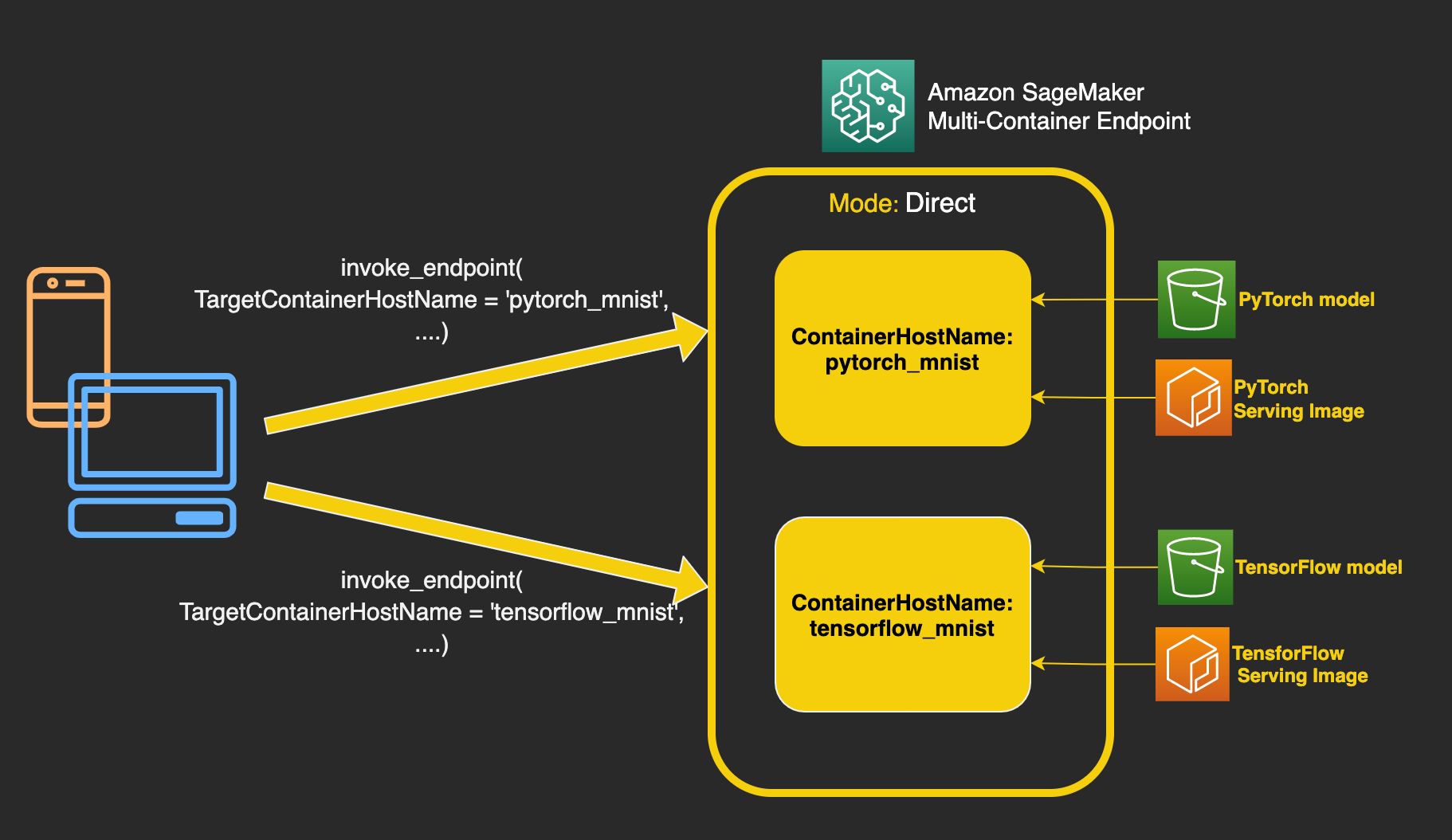
This post introduces SageMaker support for direct multi-container endpoints. This enables you to run up to 15 different ML containers on a single endpoint and invoke them independently, thereby saving up to 90% in costs. These ML containers can be running completely different ML frameworks and algorithms for model serving. In this post, we show how to serve TensorFlow and PyTorch models from the same endpoint by invoking different containers for each request and restricting access to each container.
SageMaker already supports deploying thousands of ML models and serving them using a single container and endpoint with multi-model endpoints. SageMaker also supports deploying multiple models built on different framework containers on a single instance, in a serial implementation fashion using inference pipelines.
Organizations are increasingly taking advantage of ML to solve various business problems and running different ML frameworks and algorithms for each use case. This pattern requires you to manage the challenges around deployment and cost for different serving stacks in production. These challenges become more pronounced when models are accessed infrequently but still require low-latency inference. SageMaker multi-container endpoints enable you to deploy up to 15 containers on a single endpoint and invoke them independently. This option is ideal when you have multiple models running on different serving stacks with similar resource needs, and when individual models don’t have sufficient traffic to utilize the full capacity of the endpoint instances.
Overview of SageMaker multi-container endpoints
SageMaker multi-container endpoints enable several inference containers, built on different serving stacks (such as ML framework, model server, and algorithm), to be run on the same endpoint and invoked independently for cost savings. This can be ideal when you have several different ML models that have different traffic patterns and similar resource needs.
Examples of when to utilize multi-container endpoints include, but are not limited to, the following:
- Hosting models across different frameworks (such as TensorFlow, PyTorch, and Sklearn) that don’t have sufficient traffic to saturate the full capacity of an instance
- Hosting models from the same framework with different ML algorithms (such as recommendations, forecasting, or classification) and handler functions
- Comparisons of similar architectures running on different framework versions (such as TensorFlow 1.x vs. TensorFlow 2.x) for scenarios like A/B testing
Requirements for deploying a multi-container endpoint
To launch a multi-container endpoint, you specify the list of containers along with the trained models that should be deployed on an endpoint. Direct inference mode informs SageMaker that the models are accessed independently. As of this writing, you’re limited to up to 15 containers on a multi-container endpoint and GPU inference is not supported due to resource contention. You can also run containers on multi-container endpoints sequentially as inference pipelines for each inference if you want to make preprocessing or postprocessing requests, or if you want to run a series of ML models in order. This capability is already supported as the default behavior of the multi-container endpoints and is selected by setting the inference mode to Serial.
After the models are trained, either through training on SageMaker or a bring-your-own strategy, you can deploy them on a multi-container endpoint using the SageMaker create_model, create_endpoint_config, and create_endpoint APIs. The create_endpoint_config and create_endpoint APIs work exactly the same way as they work for single model or container endpoints. The only change you need to make is in the usage of the create_model API. The following changes are required:
- Specify a dictionary of container definitions for the
Containersargument. This dictionary contains the container definitions of all the containers required to be hosted under the same endpoint. Each container definition must specify aContainerHostname. - Set the
Modeparameter ofInferenceExecutionConfigtoDirect, for direct invocation of each container, orSerial, for using containers in a sequential order (inference pipeline). The defaultModevalue isSerial.
Solution overview
In this post, we explain the usage of multi-container endpoints with the following steps:
- Train a TensorFlow and a PyTorch Model on the MNIST dataset.
- Prepare container definitions for TensorFlow and PyTorch serving.
- Create a multi-container endpoint.
- Invoke each container directly.
- Secure access to each container on a multi-container endpoint.
- View metrics for a multi-container endpoint
The complete code related to this post is available on the GitHub repo.
Dataset
The MNIST dataset contains images of handwritten digits from 0–9 and is a popular ML problem. The MNIST dataset contains 60,000 training images and 10,000 test images. This solution uses the MNIST dataset to train a TensorFlow and PyTorch model, which can classify a given image content as representing a digit between 0–9. The models give a probability score for each digit category (0–9) and the highest probability score is taken as the output.
Train TensorFlow and PyTorch models on the MNIST dataset
SageMaker provides built-in support for training models using TensorFlow and PyTorch. To learn how to train models on SageMaker, we recommend referring to the SageMaker documentation for training a PyTorch model and training a TensorFlow model, respectively. In this post, we use TensorFlow 2.3.1 and PyTorch 1.8.1 versions to train and host the models.
Prepare container definitions for TensorFlow and PyTorch serving
SageMaker has built-in support for serving these framework models, but under the hood TensorFlow uses TensorFlow Serving and PyTorch uses TorchServe. This requires launching separate containers to serve the two framework models. To use SageMaker pre-built Deep Learning Containers, see Available Deep Learning Containers Images. Alternatively, you can retrieve pre-built URIs through the SageMaker SDK. The following code snippet shows how to build the container definitions for TensorFlow and PyTorch serving containers.
- Create a container definition for TensorFlow:
tf_ecr_image_uri = sagemaker.image_uris.retrieve(
    framework="tensorflow",
    region=region,
    version="2.3.1",
    py_version="py37",
    instance_type="ml.c5.4xlarge",
    image_scope="inference",
)

tensorflow_container = {
    "ContainerHostname": "tensorflow-mnist",
    "Image": tf_ecr_image_uri,
    "ModelDataUrl": tf_mnist_model_data,
}
Apart from ContainerHostName, specify the correct serving Image provided by SageMaker and also ModelDataUrl, which is an Amazon Simple Storage Service (Amazon S3) location where the model is present.
- Create the container definition for PyTorch:
pt_ecr_image_uri = sagemaker.image_uris.retrieve(
    framework="pytorch",
    region=region,
    version="1.8.1",
    py_version="py36",
    instance_type="ml.c5.4xlarge",
    image_scope="inference",
)

pytorch_container = {
    "ContainerHostname": "pytorch-mnist",
    "Image": pt_ecr_image_uri,
    "ModelDataUrl": pt_updated_model_uri,
    "Environment": {
        "SAGEMAKER_PROGRAM": "inference.py",
        "SAGEMAKER_SUBMIT_DIRECTORY": pt_updated_model_uri,
    },
}
For PyTorch container definition, an additional argument, Environment, is provided. It contains two keys:
- SAGEMAKER_PROGRAM – The name of the script containing the inference code required by the PyTorch model server
- SAGEMAKER_SUBMIT_DIRECTORY – The S3 URI of
tar.gzcontaining the model file (model.pth) and the inference script
Create a multi-container endpoint
The next step is to create a multi-container endpoint.
- Create a model using the
create_modelAPI:
create_model_response = sm_client.create_model(
    ModelName="mnist-multi-container",
    Containers=[pytorch_container, tensorflow_container],
    InferenceExecutionConfig={"Mode": "Direct"},
    ExecutionRoleArn=role,
)
Both the container definitions are specified under the Containers argument. Additionally, the InferenceExecutionConfig mode has been set to Direct.
- Create
endpoint_configurationusing thecreate_endpoint_configAPI. It specifies the sameModelNamecreated in the previous step:
endpoint_config = sm_client.create_endpoint_config(
    EndpointConfigName="mnist-multi-container-ep-config",
    ProductionVariants=[
        {
            "VariantName": "prod",
            "ModelName": "mnist-multi-container",
            "InitialInstanceCount": 1,
            "InstanceType": "ml.c5.4xlarge",
        },
    ],
)- Create an endpoint using the
create_endpointAPI. It contains the same endpoint configuration created in the previous step:
endpoint = sm_client.create_endpoint(
    EndpointName="mnist-multi-container-ep", EndpointConfigName="mnist-multi-container-ep-config"
)
Invoke each container directly
To invoke a multi-container endpoint with direct invocation mode, use invoke_endpoint from the SageMaker Runtime, passing a TargetContainerHostname argument that specifies the same ContainerHostname used while creating the container definition. The SageMaker Runtime InvokeEndpoint request supports X-Amzn-SageMaker-Target-Container-Hostname as a new header that takes the container hostname for invocation.
The following code snippet shows how to invoke the TensorFlow model on a small sample of MNIST data. Note the value of TargetContainerHostname:
tf_result = runtime_sm_client.invoke_endpoint(
    EndpointName="mnist-multi-container-ep",
    ContentType="application/json",
    Accept="application/json",
    TargetContainerHostname="tensorflow-mnist",
    Body=json.dumps({"instances": np.expand_dims(tf_samples, 3).tolist()}),
)
Similarly, to invoke the PyTorch container, change the TargetContainerHostname to pytorch-mnist:
pt_result = runtime_sm_client.invoke_endpoint(
    EndpointName="mnist-multi-container-ep",
    ContentType="application/json",
    Accept="application/json",
    TargetContainerHostname="pytorch-mnist",
    Body=json.dumps({"inputs": np.expand_dims(pt_samples, axis=1).tolist()}),
)
Apart from using different containers, each container invocation can also support a different MIME type.
For each invocation request to a multi-container endpoint set in direct invocation mode, only the container with TargetContainerHostname processes the request. Validation errors are raised if you specify a TargetContainerHostname that doesn’t exist inside the endpoint, or if you failed to specify a TargetContainerHostname parameter when invoking a multi-container endpoint.
Secure multi-container endpoints
For multi-container endpoints using direct invocation mode, multiple containers are co-located in a single instance by sharing memory and storage volume. You can provide users with the right access to the target containers. SageMaker uses AWS Identity and Access Management (IAM) roles to provide IAM identity-based policies that allow or deny actions.
By default, an IAM principal with InvokeEndpoint permissions on a multi-container endpoint using direct invocation mode can invoke any container inside the endpoint with the EndpointName you specify. If you need to restrict InvokeEndpoint access to a limited set of containers inside the endpoint you invoke, you can restrict InvokeEndpoint calls to specific containers by using the sagemaker:TargetContainerHostname IAM condition key, similar to restricting access to models when using multi-model endpoints.
The following policy allows InvokeEndpoint requests only when the value of the TargetContainerHostname field matches one of the specified regular expressions:
{
"Version": "2012-10-17",
"Statement": [
{
"Action": [
"sagemaker:InvokeEndpoint"
],
"Effect": "Allow",
"Resource": "arn:aws:sagemaker:region:account-id:endpoint/endpoint_name",
"Condition": {
"StringLike": {
"sagemaker:TargetContainerHostname": ["customIps*", "common*"]
}
}
}
]
}
The following policy denies InvokeEndpont requests when the value of the TargetContainerHostname field matches one of the specified regular expressions of the Deny statement:
{
    "Version": "2012-10-17",
    "Statement": [
        {
            "Action": [
                "sagemaker:InvokeEndpoint"
            ],
            "Effect": "Allow",
            "Resource": "arn:aws:sagemaker:region:account-id:endpoint/endpoint_name",
            "Condition": {
                "StringLike": {
                    "sagemaker:TargetContainerHostname": [""]
                }
            }
        },
        {
            "Action": [
                "sagemaker:InvokeEndpoint"
            ],
            "Effect": "Deny",
            "Resource": "arn:aws:sagemaker:region:account-id:endpoint/endpoint_name",
            "Condition": {
                "StringLike": {
                    "sagemaker:TargetContainerHostname": ["special"]
                }
            }
        }
    ]
}
For information about SageMaker condition keys, see Condition Keys for Amazon SageMaker.
Monitor multi-container endpoints
For multi-container endpoints using direct invocation mode, SageMaker not only provides instance-level metrics as it does with other common endpoints, but also supports per-container metrics.
Per-container metrics for multi-container endpoints with direct invocation mode are located in Amazon CloudWatch metrics and are categorized into two namespaces: AWS/SageMaker and aws/sagemaker/Endpoints. The namespace of AWS/SageMaker includes invocation-related metrics, and the aws/sagemaker/Endpoints namespace includes per-container metrics of memory and CPU utilization.
The following screenshot of the AWS/SageMaker namespace shows per-container latency.

The following screenshot shows the aws/sagemaker/Endpoints namespace, which displays the CPU and memory utilization for each container.

For a full list of metrics, see Monitor Amazon SageMaker with Amazon CloudWatch.
Conclusion
SageMaker multi-container endpoints support deploying up to 15 containers on real-time endpoints and invoking them independently for low-latency inference and cost savings. The models can be completely heterogenous, with their own independent serving stack. You can either invoke these containers sequentially or independently for each request. Securely hosting multiple models, from different frameworks, on a single instance could save you up to 90% in cost.
To learn more, see Deploy multi-container endpoints and try out the example used in this post on the SageMaker GitHub examples repo.
About the Author
 Vikesh Pandey is a Machine Learning Specialist Specialist Solutions Architect at AWS, helping customers in the Nordics and wider EMEA region design and build ML solutions. Outside of work, Vikesh enjoys trying out different cuisines and playing outdoor sports.
 Sean Morgan is an AI/ML Solutions Architect at AWS. He previously worked in the semiconductor industry, using computer vision to improve product yield. He later transitioned to a DoD research lab where he specialized in adversarial ML defense and network security. In his free time, Sean is an active open-source contributor and maintainer, and is the special interest group lead for TensorFlow Addons.
Machine Learning at the Edge with AWS Outposts and Amazon SageMaker
As customers continue to come up with new use-cases for machine learning, data gravity is as important as ever. Where latency and network connectivity is not an issue, generating data in one location (such as a manufacturing facility) and sending it to the cloud for inference is acceptable for some use-cases. With other critical use-cases, such as fraud detection for financial transactions, product quality in manufacturing, or analyzing video surveillance in real-time, customers are faced with the challenges that come with having to move that data to the cloud first. One of the challenges customers are facing with performing inference in the cloud is the lack of real-time inference and/or security requirements preventing user data to be sent or stored in the cloud.
Tens of thousands of customers use Amazon SageMaker to accelerate their Machine Learning (ML) journey by helping data scientists and developers to prepare, build, train, and deploy machine learning models quickly. Once you’ve built and trained your ML model with SageMaker, you’ll want to deploy it somewhere to start collecting inputs to run through your model (inference). These models can be deployed and run on AWS, but we know that there are use-cases that don’t lend themselves well for running inference in an AWS Region while the inputs come from outside the Region. Cases include a customer’s data center, manufacturing facility, or autonomous vehicles. Predictions must be made in real-time when new data is available. When you want to run inference locally or on an edge device, a gateway, an appliance or on-premises server, you can optimize your ML models for the specific underlying hardware with Amazon SageMaker Neo. It is the easiest way to optimize ML models for edge devices, enabling you to train ML models once in the cloud and run them on any device. To increase efficiency of your edge ML operations, you can use Amazon SageMaker Edge Manager to automate the manual steps to optimize, test, deploy, monitor and maintain your models on fleets of edge devices.
In this blog post, we will talk about the different use-cases for inference at the edge and the way to accomplish it using Amazon SageMaker features and AWS Outposts. Let’s review each, before we dive into ML with AWS Outposts.
Amazon SageMaker – Amazon SageMaker is a fully managed service that provides every developer and data scientist with the ability to build, train, and deploy machine learning (ML) models quickly. SageMaker removes the heavy lifting from each step of the machine learning process to make it easier to develop high quality models.
Amazon SageMaker Edge Manager – Amazon SageMaker Edge Manager provides a software agent that runs on edge devices. The agent comes with a ML model optimized with SageMaker Neo automatically. You don’t need to have Neo runtime installed on your devices in order to take advantage of the model optimizations such as machine learning models performing at up to twice the speed with no loss in accuracy. Other benefits include reduction of hardware resource usage by up to 10x and the ability to run the same ML model on multiple hardware platforms. The agent also collects prediction data and sends a sample of the data to the AWS Region for monitoring, labeling, and retraining so you can keep models accurate over time.
AWS Outposts – AWS Outposts is a fully managed service that offers the same AWS infrastructure, AWS services, APIs, and tools to virtually any data center, co-location space, or on-premises facility for a truly consistent hybrid experience. AWS Outposts is ideal for workloads that require low latency access to on-premises systems, local data processing, data residency, and migration of applications with local system interdependencies.
AWS compute, storage, database, and other services run locally on Outposts. You can access the full range of AWS services available in the Region to build, manage, and scale your on-premises applications using familiar AWS services and tools.
Use cases
Due to low latency needs or large volumes of data, customers need ML inferencing at the edge. Two main use-cases require customers to implement these models for inference at the edge:
Low Latency – In many use-cases, the end user or application must provide inferencing in (near) real-time, requiring the model to be running at the edge. This is a common use case in industries such as Financial Services (risk analysis), Healthcare (medical imaging analysis), Autonomous Vehicles and Manufacturing (shop floor).
Large Volumes of Data – Large volumes of new data being generated at the edge means that inferencing needs to happen closer to where data is being generated. This is a common use case in IoT scenarios, such as in the oil and gas or utilities industries.
Scenario
For this scenario, let’s focus on the low latency use-case. A financial services customer wants to implement fraud detection on all customer transactions. They’ve decided on using Amazon SageMaker to build and train their model in an AWS Region. Given the distance between the data center in which they process transactions and an AWS Region, inference needs to be performed locally, in the same location as the transaction processing. They will use Amazon SageMaker Edge Manager to optimize the trained model to perform inference locally in their data center. The last piece is the compute. The customer is not interested in managing the hardware and their team is already trained in AWS development, operations and management. Given that, the customer chose AWS Outposts as their compute to run locally in their data center.
What does this look like technically? Let’s take a look at an architecture and then talk through the different pieces.
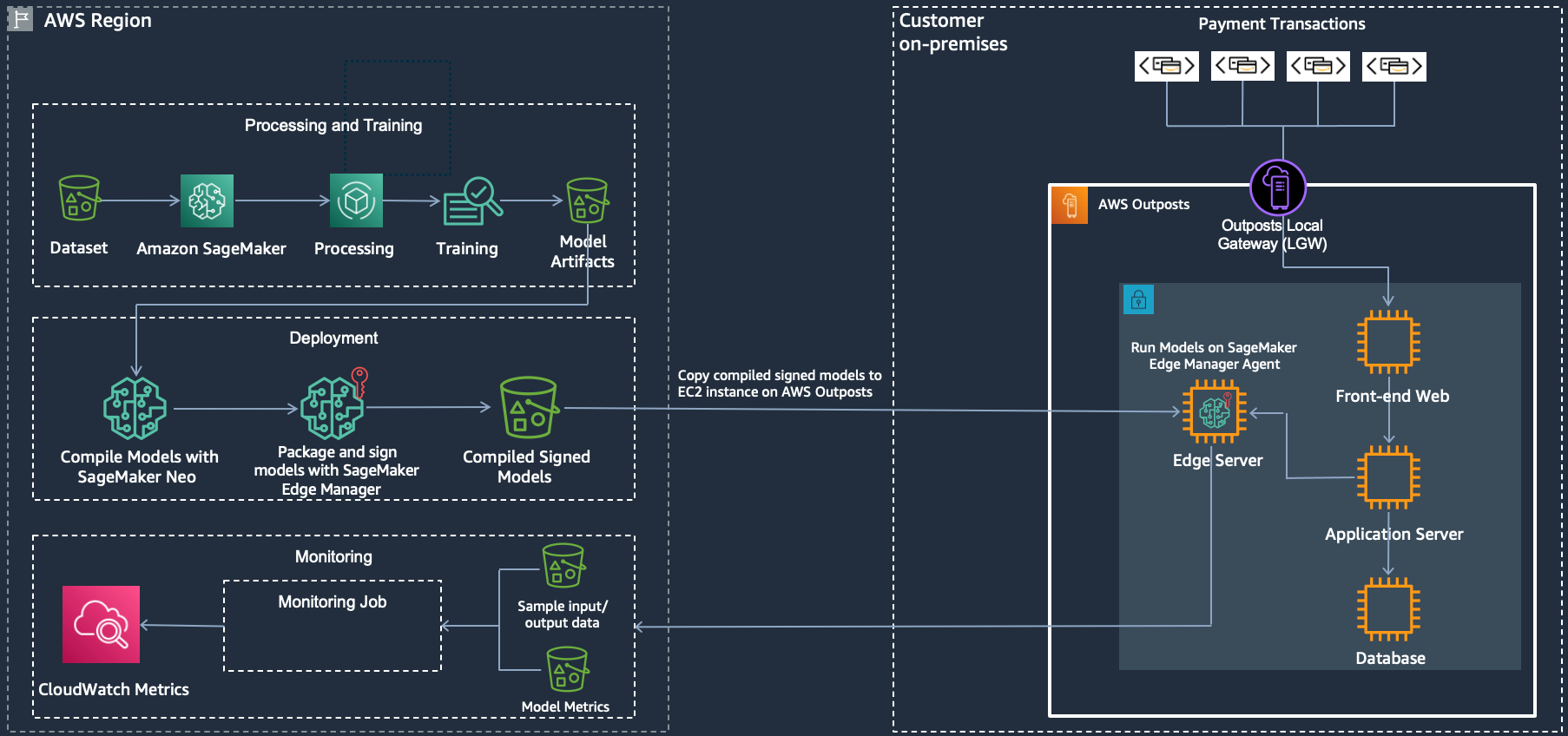
Let’s look at the flow. On the left, training of the model is done in the AWS Region with Amazon SageMaker for training and packaging. On the right, we have a data center, which can be the customer data center or a co-location facility, with AWS Outposts and SageMaker Edge Manager to do the inference.
AWS Region:
- Load dataset into Amazon S3, which acts as input for model training.
- Use Amazon SageMaker to do processing and training against the dataset.
- Store the model artifacts in Amazon S3.
- Compile the trained model using Amazon SageMaker Neo.
- Package and sign the model with Amazon SageMaker Edge Manger and store in Amazon S3.
AWS Outposts
- Launch an Amazon EC2 instance (use the instance family that you’ve optimized the model for) in a subnet that lives on the AWS Outposts.
- Install Amazon SageMaker Edge Manager agent onto the instance. Learn more about installing the agent here.
- Copy the compiled and signed model from Amazon S3 in the AWS Region to the Amazon EC2 instance on the AWS Outposts. Here’s an example using the AWS CLI to copy a model file (model-ml_m5.tar.gz) from Amazon S3 to the current directory (.):
aws s3 cp s3://sagemaker-studio-66f50fg898c/fraud-detection-ml/profiler/model-ml_m5.tar.gz .
- Financial transactions come into the data center and are routed into the Outposts via the Local Gateway (LGW), to the front-end web server and then to the application server.
- The transaction gets stored in the database and at the same time, the application server generates a customer profile based on multiple variables, including transaction history.
- The customer profile is sent to Edge Manager agent to run inference against the compiled model using the customer profile as input.
- The fraud detection model will generate a score once inference is complete. Based on that score the application server will return one of the following back to the client:
- Approve the transaction.
- Ask for 2nd factor (two factor authentication).
- Deny the transaction.
- Additionally, sample input/output data as well as model metrics are captured and sent back to the AWS Region for monitoring with Amazon SageMaker Edge Manager.
AWS Region
- Monitor your model with Amazon SageMaker Edge Manager and push metrics in to CloudWatch, which can be used as a feedback loop to improve the model’s performance on an on-going basis.
Considerations for Using Amazon SageMaker Edge Manager with AWS Outposts
Factors to consider when choosing between inference in an AWS Region vs AWS Outposts:
- Security: Whether other factors are relevant to your use-case or not, security of your data is a priority. If the data you must perform inference on is not permissible to be stored in the cloud, AWS Outposts for inference at the edge will perform inference without sacrificing data security.
- Real-time processing: Is the data you need to perform inference on time bound? If the value of the data diminishes as more time passes, then sending the data to an AWS Region for inference may not have value.
- WAN Connectivity: Along with the speed and quality of your connection, the time from where the data is generated and sent to the cloud (latency) is also important. You may only need near real-time inference and cloud-based inference is an option.
- Do you have enough bandwidth to send the amount of data back to an AWS Region? If not, is the required bandwidth cost effective?
- Is the quality of network link back to the AWS Region suitable to meet your requirements?
- What are the consequences of a network outage?
If link quality is an issue, if bandwidth costs are not reasonable, or a network outage is detrimental to your business, then using AWS Outposts for inference at the edge can help to ensure that you’re able to continually perform inference regardless of the state of your WAN connectivity.
As of the writing of this blog post, Amazon SageMaker Edge Manager supports common CPU (ARM, x86), GPU (ARM, Nvidia) based devices with Linux and Windows operating systems. Over time, SageMaker Edge Manager will expand to support more embedded processors and mobile platforms that are also supported by SageMaker Neo.
Additionally, you need to use Amazon SageMaker Neo to compile the model in order to use Amazon SageMaker Edge Manager. Amazon SageMaker Neo converts and compiles your models into an executable that you can then package and deploy on to your edge devices. Once the model package is deployed, Amazon SageMaker Edge Manager agent will unpack the model package and run the model on the device.
Conclusion
Whether it’s providing quality assurance to manufactured goods, real-time monitoring of cameras, wind farms, or medical devices (and countless other use-cases), Amazon SageMaker combined with AWS Outposts provides you with world class machine learning capabilities and inference at the edge.
To learn more about Amazon SageMaker Edge Manager, you can visit the Edge Manager product page and check out this demo. To learn more about AWS Outposts, visit the Outposts product page and check out this introduction.
About the Author
 Josh Coen is a Senior Solutions Architect at AWS specializing in AWS Outposts. Prior to joining AWS, Josh was a Cloud Architect at Sirius, a national technology systems integrator, where he helped build and run their AWS practice. Josh has a BS in Information Technology and has been in the IT industry since 2003.
 Mani Khanuja is an Artificial Intelligence and Machine Learning Specialist SA at Amazon Web Services (AWS). She helps customers use machine learning to solve their business challenges using AWS. She spends most of her time diving deep and teaching customers on AI/ML projects related to computer vision, natural language processing, forecasting, ML at the edge, and more. She is passionate about ML at edge and has created her own lab with a self-driving kit and prototype manufacturing production line, where she spends a lot of her free time.
Alexa Prize faculty advisors provide insights on the competition
Teams’ research papers that outline their approaches to development and deployment are now available.Read More
Czech Technical University team wins Alexa Prize SocialBot Grand Challenge 4
Team Alquist awarded $500,000 prize for top score in finals competition; teams from Stanford University and the University of Buffalo place second and third.Read More
Pose estimation and classification on edge devices with MoveNet and TensorFlow Lite

Posted by Khanh LeViet, TensorFlow Developer Advocate and Yu-hui Chen, Software Engineer
Since MoveNet’s announcement at Google I/O earlier this year, we have received a lot of positive feedback and feature requests. Today, we are excited to share several updates with you:
- The TensorFlow Lite version of MoveNet is now available on TensorFlow Hub. This includes a few updates to improve accuracy and make it compatible with hardware accelerators including GPUs and other accelerators available via the Android NN API.
- We’ve released a new Android, Raspberry Pi pose estimation sample that lets you try out MoveNet on mobile and IoT devices. (iOS is coming soon)
- We’ve also released a Colab notebook that teaches you how to do custom pose classification (e.g. recognize different yoga poses) with MoveNet. You can try pose classification on the Android, iOS and Raspberry Pi apps mentioned earlier.
What is pose estimation?
Pose estimation is a machine learning task that estimates the pose of a person from an image or a video by estimating the spatial locations of specific body parts (keypoints). MoveNet is the state-of-the-art pose estimation model that can detect these 17 key-points:
- Nose
- Left and right eye
- Left and right ear
- Left and right shoulder
- Left and right elbow
- Left and right wrist
- Left and right hip
- Left and right knee
- Left and right ankle
We have released two versions of MoveNet:
- MoveNet.Lightning is smaller, faster but less accurate than the Thunder version. It can run in realtime on modern smartphones.
- MoveNet.Thunder is the more accurate version but also larger and slower than Lightning.
The MoveNet models outperform Posenet (paper, blog post, model), our previous TensorFlow Lite pose estimation model, on a variety of benchmark datasets (see the evaluation/benchmark result in the table below).
These MoveNet models are available in both the TensorFlow Lite FP16 and INT8 quantized formats, allowing maximum compatibility with hardware accelerators.
This version of MoveNet can recognize a single pose from the input image. If there is more than one person in the image, the model along with the cropping algorithm will try its best to focus on the person who is closest to the image center. We have also implemented a smart cropping algorithm to improve the detection accuracy on videos. In short, the model will zoom into the region where there’s a pose detected in the previous frame, so that the model can see the finer details and make better predictions in the current frame.
If you are interested in a deep-dive into MoveNet’s implementation details, check out an earlier blog post including its model architecture and the dataset it was trained on.
Sample app for Android and Raspberry Pi
We have released new pose estimation sample apps for these platforms so that you can quickly try out different pose estimation models (MoveNet Lightning, MoveNet Thunder, Posenet) on the platform of your choice.
- Android sample
- iOS sample
- Raspberry Pi sample
In the Android and iOS sample, you can also choose an accelerator (GPU, NNAPI, CoreML) to run the pose estimation models.
 |
|
Screenshot of the Android sample app. The image is from Pixabay. |
MoveNet performance
We have optimized MoveNet to run well on hardware accelerators supported by TensorFlow Lite, including GPU and accelerators available via the Android NN API. This performance benchmark result may help you choose the runtime configurations that are most suitable for your use cases.
|
Model |
Size (MB) |
mAP* |
Latency (ms) ** |
||
|
Pixel 5 – |
Pixel 5 – GPU |
Raspberry Pi 4 – CPU 4 threads |
|||
|
MoveNet.Thunder (FP16 quantized) |
12.6MB |
72.0 |
155ms |
45ms |
594ms |
|
MoveNet.Thunder (INT8 quantized) |
7.1MB |
68.9 |
100ms |
52ms |
251ms |
|
MoveNet.Lightning (FP16 quantized) |
4.8MB |
63.0 |
60ms |
25ms |
186ms |
|
MoveNet.Lightning (INT8 quantized) |
2.9MB |
57.4 |
52ms |
28ms |
95ms |
|
PoseNet |
13.3MB |
45.6 |
80ms |
40ms |
338ms |
* mAP was measured on a subset of the COCO keypoint dataset where we filter and crop each image to contain only one person.
** Latency was measured end-to-end using the Android and Raspberry Pi sample apps with TensorFlow 2.5 under sustained load.
Here are some tips when deciding which model and accelerator to use:
- Choose Lightning or Thunder. Firstly, you should see whether the accuracy of the Lightning version is enough for your use case.
- If the Lightning INT8 model’s accuracy is good enough, then go with it because it’s the smallest and fastest model in the lineup. A faster model also means less battery consumed.
- If having good accuracy is critical for your use case, go with the Thunder FP16 model.
- Choose the accelerator. Accelerator performance varies a lot between Android devices from different manufacturers.
- CPU is the safest and simplest choice because you can know for sure that it will work on practically any Android device that can run TensorFlow Lite. However, it is usually slower and consumes more power than running the model on accelerators. All MoveNet models can run well on CPU so you should choose a model based on your accuracy needs.
- GPU is the most widely available accelerator and provides a decent performance boost. Choose the FP16 quantized models if you want to leverage GPUs.
- Android NNAPI is the convenient way to access additional ML accelerators on Android devices. If you are already using the CPU or GPU for other workloads and your user’s device runs Android 10 or a newer version, you can choose a model that suits your accuracy needs, and let NNAPI choose the path that it thinks works best for your model.
- If you are an IoT developer, you may want to use Coral to increase inference speed. See the benchmark numbers for Coral here.
- Deploy the model over-the-air rather than bundle it in the app binary. Due to the variety of the Android ecosystem, there’s no single model that is optimal for all of your users. For users with lower-end devices, the Lightning INT8 model might be optimal for them because it’s the fastest and consumes the least battery. However, for users with high-end devices, you may want to deliver better performance using the Thunder FP16 model. If you want to change models according to the user device, consider using the free Firebase ML to host your models instead of bundling all the models you intend to use into your app. You can write a logic to download an optimal model for each of your user’s device when the user starts using a feature in your app that requires the TFLite model.
Pose classification
While the pose estimation model tells you where the pose key points are, in many fitness applications, you may want to go further and classify the pose, for example whether it’s a yoga goddess pose or a plank pose, to deliver relevant information to your users.
To make pose classification easier to implement, we’ve also released a Colab notebook that teaches you how to use MoveNet and TensorFlow Lite to train a custom pose classification model from your custom pose dataset. It means that if you want to recognize yoga poses, all you need is to collect images of poses that you want to recognize, label them, and follow the tutorial to train and deploy a yoga pose classifier into your applications.
The pose classifier consists of two stages:
- Use MoveNet to detect keypoints from the input image.
- Use a small TensorFlow Lite model to classify the pose from the detected keypoints.
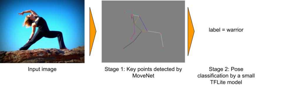 |
|
An example of pose classification using MoveNet. The input image is from Pixabay. |
In order to train a custom pose classifier, you need to prepare the pose images and put them into a folder structure as below. Each subfolder name is the name of the class you want to recognize. Then you can run the notebook to train a custom pose classifier and convert it to the TensorFlow Lite format.
yoga_poses
|__ downdog
    |______ 00000128.jpg
    |______ 00000181.bmp
    |______ ...
|__ goddess
    |______ 00000243.jpg
    |______ 00000306.jpg
    |______ ...
...
The pose classification TensorFlow Lite model is very small, only about 30KBs. It takes the landmarks output from MoveNet, normalizes the pose coordinates and feeds it through a few fully connected layers. The model output is a list of probabilities that the pose is each of the known pose types.
 |
| Overview of the pose classification TensorFlow Lite model. |
You can try your pose classification model in any of the pose estimation sample apps for Android or Raspberry Pi that we have just released.
What’s next
Our goal is to provide the core pose estimation and action recognition engine so that developers can build creative applications on top of it. Here are some of the directions that we are actively working on:
- An improved version of MoveNet that can detect multiple poses in one forward path.
- Action recognition based on the detected poses on multiple frames.
Please let us know via tflite@tensorflow.org or the TensorFlow Forum if you have any feedback or suggestions!
Acknowledgements
We would like to thank the other contributors to MoveNet: Ronny Votel, Ard Oerlemans, Francois Belletti along with those involved with the TensorFlow Lite: Tian Lin, Lu Wang.
What Is a Machine Learning Model?
When you shop for a car, the first question is what model — a Honda Civic for low-cost commuting, a Chevy Corvette for looking good and moving fast, or maybe a Ford F-150 to tote heavy loads.
For the journey to AI, the most transformational technology of our time, the engine you need is a machine learning model.
What Is a Machine Learning Model?
A machine learning model is an expression of an algorithm that combs through mountains of data to find patterns or make predictions. Fueled by data, machine learning (ML) models are the mathematical engines of artificial intelligence.
For example, an ML model for computer vision might be able to identify cars and pedestrians in a real-time video. One for natural language processing might translate words and sentences.
Under the hood, a model is a mathematical representation of objects and their relationships to each other. The objects can be anything from “likes” on a social networking post to molecules in a lab experiment.
ML Models for Every Purpose
With no constraints on the objects that can become features in an ML model, there’s no limit to the uses for AI. The combinations are infinite.
Data scientists have created whole families of machine learning models for different uses, and more are in the works.
A Brief Taxonomy of ML Models
| ML Model Type | Uses Cases |
|---|---|
| Linear regression/classification | Patterns in numeric data, such as financial spreadsheets |
| Graphic models | Fraud detection or sentiment awareness |
| Decision trees/Random forests | Predicting outcomes |
| Deep learning neural networks | Computer vision, natural language processing and more |
For instance, linear models use algebra to predict relationships between variables in financial projections. Graphical models express as diagrams a probability, such as whether a consumer will choose to buy a product. Borrowing the metaphor of branches, some ML models take the form of decision trees or groups of them called random forests.
In the Big Bang of AI in 2012, researchers found deep learning to be one of the most successful techniques for finding patterns and making predictions. It uses a kind of machine learning model called a neural network because it was inspired by the patterns and functions of brain cells.
An ML Model for the Masses
Deep learning took its name from the structure of its machine learning models. They stack layer upon layer of features and their relationships, forming a mathematical hero sandwich.
Thanks to their uncanny accuracy in finding patterns, two kinds of deep learning models, described in a separate explainer, are appearing everywhere.
Convolutional neural networks (CNNs), often used in computer vision, act like eyes in autonomous vehicles and can help spot diseases in medical imaging. Recurrent neural networks and transformers (RNNs), tuned to analyze spoken and written language, are the engines of Amazon’s Alexa, Google’s Assistant and Apple’s Siri.

Pssssst, Pick a Pretrained Model
Choosing the right family of models — like a CNN, RNN or transformer — is a great beginning. But that’s just the start.
If you want to ride the Baja 500, you can modify a stock dune buggy with heavy duty shocks and rugged tires, or you can shop for a vehicle built for that race.
In machine learning, that’s what’s called a pretrained model. It’s tuned on large sets of training data that are similar to data in your use case. Data relationships — called weights and biases — are optimized for the intended application.
It takes an enormous dataset, a lot of AI expertise and significant compute muscle to train a model. Savvy buyers shop for pretrained models to save time and money.
Who Ya Gonna Call?
When you’re shopping for a pretrained model, find a dealer you can trust.
NVIDIA puts its name behind an online library called the NGC catalog that’s filled with vetted, pretrained models. They span the spectrum of AI jobs from computer vision and conversational AI and more.
Users know what they’re getting because models in the catalog come with résumés. They’re like the credentials of a prospective hire.
Model resumes show you the domain the model was trained for, the dataset that trained it, and how it’s expected to perform. They provide transparency and confidence you’re picking the right model for your use case.
More Resources for ML Models
What’s more, NGC models are ready for transfer learning. That’s the one final tune-up that torques models for the exact road conditions over which they’ll ride — your application’s data.
NVIDIA even provides the wrench to tune your NGC model. It’s called TAO and you can sign up for early access to it today.
To learn more, check out:
- Our web page on pretrained models
- A guide to the NGC catalog
- Our web page on Tao and related tools
- A developer blog on using pretrained models for computer vision to build a gesture recognition app
- A talk from GTC 21 on transfer learning (free to view with registration)
The post What Is a Machine Learning Model? appeared first on The Official NVIDIA Blog.
Supporting COVID-19 policy response with large-scale mobility-based modeling
Mobility restrictions, from stay-at-home orders to indoor occupancy caps, have been utilized extensively by policymakers during the COVID-19 pandemic. These reductions in mobility help to control the spread of the virus 12, but they come at a heavy cost to businesses and employees.
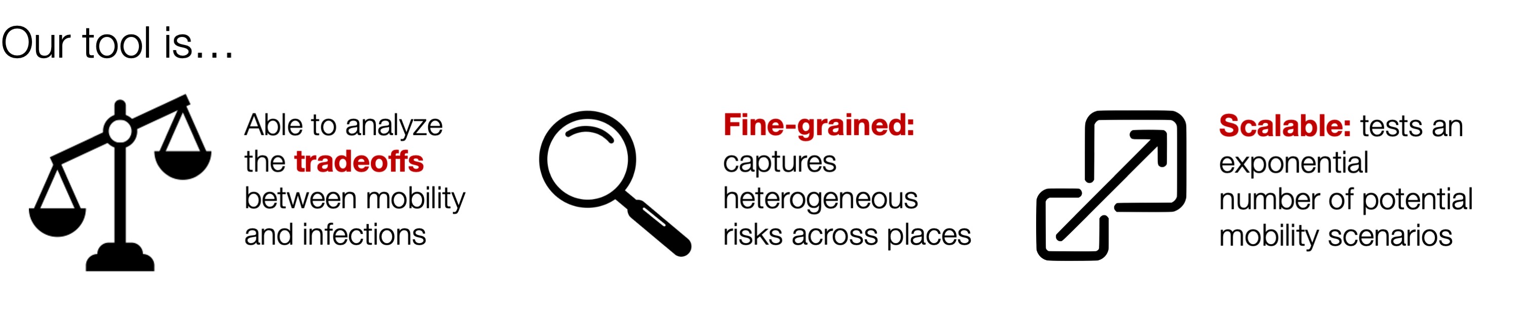
To balance these competing demands, policymakers need analytical tools that can evaluate the tradeoffs between mobility and COVID-19 infections. Furthermore, such tools should be fine-grained, able to test out heterogeneous plans—for example, allowing one level of mobility at essential retail, another level at gyms, and yet another at restaurants—so that policymakers can tailor restrictions to the specific risks and needs of each sector. At the same time, the tool also needs to be scalable, supporting analyses for a massive number of potential policies so that policymakers can find the best option for their jurisdiction.
Our tool
To fulfill these needs, we developed a novel computational tool, which we built in collaboration with the Biocomplexity Institute & Initiative at UVA to support the Virginia Department of Health (VDH). Described in our award-winning KDD 2021 paper, our tool enables policymakers to assess the costs and benefits of thousands of different mobility measures, based on millions of simulations from our underlying epidemiological model. We designed our tool to fulfill VDH’s desire to have a quantitative and comprehensive analysis of a range of reopening policies. With their guidance, we developed an interactive dashboard, where policymakers can select various proposed changes in mobility and observe their predicted impacts on COVID-19 infections over time and across regions.
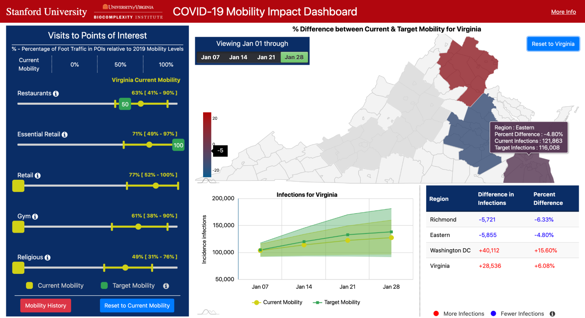
Our dashboard focuses on mobility to five key categories of places: Restaurants, Gyms, Religious Organizations, Essential Retail (grocery stores, pharmacies, convenience stores), and Retail (clothing stores, book stores, hardware stores, etc.). For each category, the user can use sliders to choose a target level of mobility (e.g., 50% of normal levels, based on pre-pandemic mobility), or they can choose to continue current levels of mobility at these places. The other panels on the dashboard then visualize predicted COVID-19 infections under the selected mobility plan, and compare these outcomes to what would happen if all categories remained at their current levels of mobility.
Our tool enables policymakers to comprehensively analyze pandemic tradeoffs, by quantifying visits lost under each mobility plan as well as predicted infections. The sliders for each category allow them to test fine-grained, heterogeneous policies. Furthermore, the flexibility of our approach (i.e., allowing any combination of mobility levels) results in an exponential number of scenarios to test. To scale our modeling efforts, our tool features a robust computational infrastructure that compresses 2 years of compute time into the span of a few days.
Our approach
At the heart of our tool is our state-of-the-art epidemiological model which utilizes large-scale mobility networks to accurately capture the spread of COVID-19 in cities across the US.
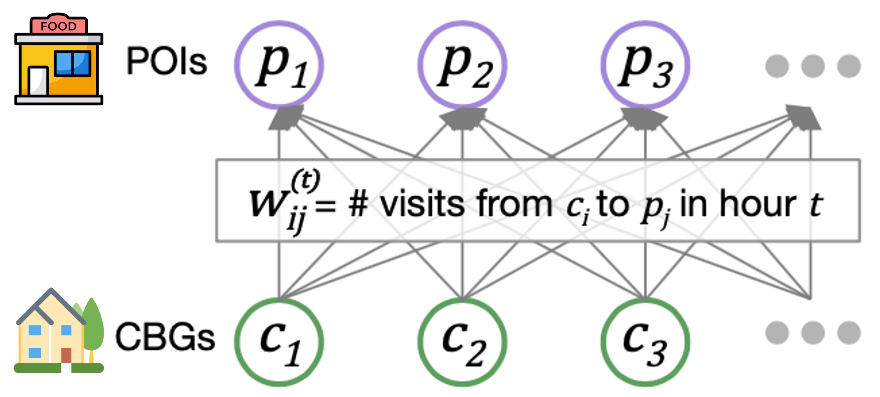
Our mobility networks encode the hourly movements of people from census block groups (CBGs) to points of interest (POIs), which are non-residential locations such as restaurants, grocery stores, and churches. Using iterative proportional fitting, we infer these networks from aggregated, anonymized location data provided by SafeGraph. In this work, we infer hourly networks for the Washington DC, Virginia Beach, and Richmond metropolitan areas, three of the largest metropolitan areas in Virginia. From November 1 to December 31, 2020, their resulting networks contain 3.4 billion hourly edges between CBGs and POIs.
We integrate the mobility networks, along with other data sources such as daily mask use, into our model. The key to our model is that it maintains the number of people in each CBG who are susceptible (S), exposed (E), infectious (I), or removed (R).

These CBG states are updated in each hour of the simulation, based on transmission dynamics that capture both household transmission and transmission occurring at POIs. That is, if there are susceptible and infectious individuals visiting a POI at the same time, then we model some probability of new infection occurring. That probability depends on the POI’s area in square feet, its median dwell time, the percentage of people wearing masks, and the number of susceptible and infectious visitors. Based on all of these factors, our model realistically captures who was infected where and when, down to the individual POI and hour.
To validate our models, we compare its predictions against actual daily COVID-19 cases and deaths, as reported by The New York Times. In our initial work 3, published in Nature 2020, we showed that our dynamic mobility networks enable even these relatively simple SEIR models with minimal free parameters to accurately fit real case trajectories and predict case counts in held-out time periods, despite substantial changes in population behavior during the pandemic. Integrating these networks furthermore allows us to capture the fine-grained spread of the virus, enabling analyses of the riskiest venues to reopen and the most at-risk populations.
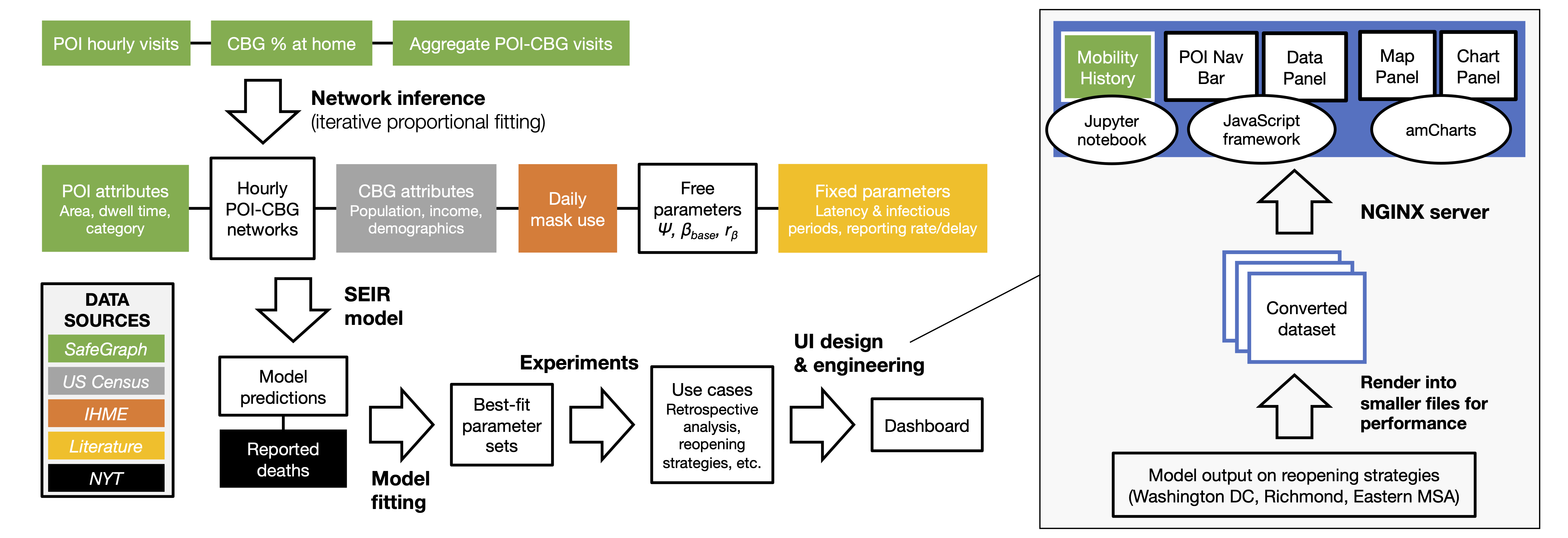
In this work, we sought to translate our model into a tool that can directly support COVID-19 decision-makers, motivated by our interactions with the Virginia Department of Health. This goal required many extensions to our computational pipeline, including fitting the model to new regions and time periods, and improving our computational infrastructure to deploy the model at scale. Furthermore, to keep pace with developments in the pandemic, we introduced new real-world features to the model such as daily mask use, time-varying case and death detection rates, and model initialization based on historical reported cases/deaths. These additions allowed us to accurately fit real COVID-19 trajectories in Virginia, and we showed that the inclusion of our new features contributed substantially toward reducing model loss. Most importantly, we worked with VDH to design use cases of our model that were most relevant to their needs, and developed a new dashboard to effectively communicate thousands of results from our model. Our full pipeline—the extended model, the computational infrastructure, and the new dashboard—constitutes advancements in this work that allowed us to truly transform our scientific model into a tool for real-world impact.
Using our model
Our fitted model can be applied to a wide variety of use cases. First, we can use it for retrospective analyses, by leveraging the model’s ability to capture who got infected where and when.
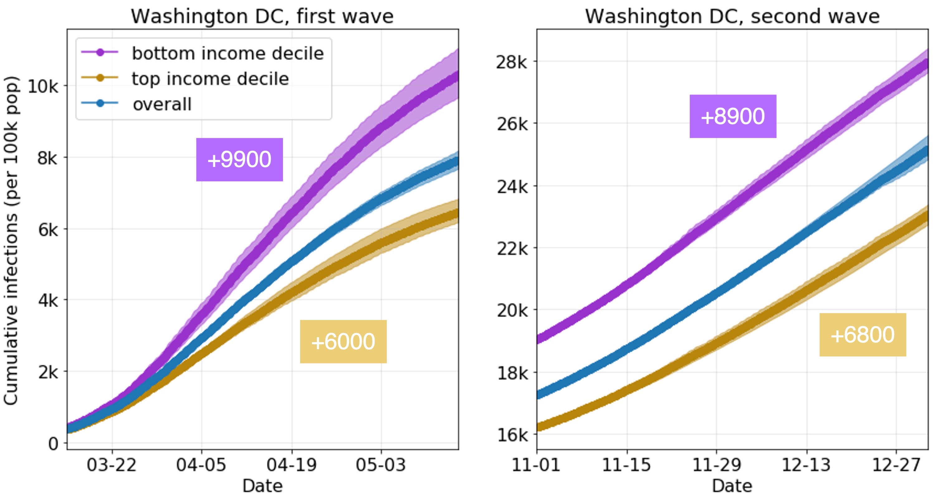
For example, we can use the model to compare the learned infection rates of lower-income and higher-income CBGs. What’s striking is that our model correctly predicts disparities from mobility data alone, even though we did not give our model any CBG demographics during runtime (only during analysis). In our prior work, we showed that two mechanisms in the mobility data explained these predicted disparities: lower-income CBGs were not able to reduce their mobility as much during the pandemic, and the POIs that they go to (even in the same category) tend to be more crowded with longer visits, and thus riskier. In this work, we show that this trend extends to both waves of the pandemic and to new metropolitan areas.
We can also use the model for forward-facing experiments. Essentially, the model has many different interpretable inputs, so we can simply modify one of those inputs, run the model, and observe what happens to the model’s predicted infections. For example, to generate data for our dashboard, we modify the mobility networks to reflect the user’s selected levels of mobility for each category, and run the model forward to produce predicted infections. We can also use our model to analyze vaccination strategies; for example, by reducing transmission rates per CBG based on the percentage of the CBG that is vaccinated.
Discussion & next steps
Our approach is not without its limitations, which we have discussed with policymakers. For instance, the mobility data from SafeGraph does not cover all POIs (e.g., limited coverage of nursing homes) or populations (e.g., children), and our model makes necessary but simplifying assumptions about the dynamics of disease transmission. Furthermore, in this work, we focused on how changes in mobility impact transmission, but where do these changes in mobility come from and how can we effect them? In future work, we plan to develop new models to answer these questions, to analyze and predict how complex mobility networks change in response to policy interventions and other pandemic events.
That said, in this work we’ve addressed a significant part of the puzzle, by introducing a tool that provides a quantitative and comprehensive near real-time assessment of the effects of mobility on transmission. Our underlying model is furthermore capable of many more types of analyses, from informing inequities to evaluating future vaccination strategies. In fact, we are now supporting the Virginia Department of Health on their vaccination efforts and extending our model to evaluate different vaccination policies. As the pandemic evolves, we will continue building decision-support tools and advancing the capabilities of our model, so that we can best support the needs of policymakers.
Acknowledgements
Special thanks to the SAIL blog editors, Emma Pierson, and Pang Wei Koh for their helpful feedback on this post. This blog post is based on our paper in KDD 2021:
Supporting COVID-19 policy response with large-scale mobility-based modeling. Serina Chang, Mandy L. Wilson, Bryan Lewis, Zakaria Mehrab, Komal K. Dudakiya, Emma Pierson, Pang Wei Koh, Jaline Gerardin, Beth Redbird, David Grusky, Madhav Marathe, and Jure Leskovec. KDD 2021 (Applied Data Science Track, Best Paper Award).
-
S. Gao, J. Rao, Y. Kang, et al. Association of mobile phone location data indications of travel and stay-at-home mandates with COVID-19 infection rates in the US. JAMA Netw Open (2020). ↩
-
J. Oh, HY. Lee, Q. Khuong, et al. Mobility restrictions were associated with reductions in COVID-19 incidence early in the pandemic: evidence from a real-time evaluation in 34 countries. Sci Rep 11, 13717 (2021). ↩
-
S. Chang, E. Pierson, P.W. Koh, et al. Mobility network models of COVID-19 explain inequities and inform reopening. Nature 589, 82–87 (2020). ↩
NVIDIA Brings Metaverse Momentum, Research Breakthroughs and New Pro GPU to SIGGRAPH
Award-winning research, stunning demos, a sweeping vision for how NVIDIA Omniverse will accelerate the work of millions more professionals, and a new pro RTX GPU were the highlights at this week’s SIGGRAPH pro graphics conference.
Kicking off the week, NVIDA’s SIGGRAPH special address featuring Richard Kerris, vice president, Omniverse, and Sanja Fidler, senior director, AI research, with an intro by Pixar co-founder Alvy Ray Smith gathered more than 1.6 million views in just 48 hours.
A documentary launched Wednesday, “Connecting in the Metaverse: The Making of the GTC Keynote” – a behind-the-scenes view into how a small team of artists were able to blur the lines between real and rendered in NVIDIA’s GTC21 keynote achieved more than 360,000 views within the first 24 hours.
In all, NVIDIA brought together professionals from every corner of the industry, hosting over 12 sessions and launching 22 demos this week.
Among the highlights:
- NVIDIA announced a major expansion of NVIDIA Omniverse — the world’s first simulation and collaboration platform — through new integrations with Blender and Adobe that will open it to millions more users.
- NVIDIA’s research team took the coveted SIGGRAPH Best of Show award for a stunning new demo.
- And NVIDIA’s new NVIDIA RTX A2000 GPU, announced this week, will expand the availability of RTX technology to millions more pros.
It was a week packed with innovations, many captured in a new sizzle reel crammed with new technologies.
Sessions from the NVIDIA Deep Learning Institute brought the latest ideas to veteran developers and students alike.
And the inaugural gathering of the NVIDIA Omniverse User Group brought more than 400 graphics professionals from all over the world together to learn about what’s coming next for Omniverse, to celebrate the work of the community, and announce the winners of the second #CreatewithMarbles: Marvelous Machine contest.
“Your work fuels what we do,” Rev Lebaredian, vice president of Omniverse engineering and simulation at NVIDIA told the scores of Omniverse users gathered for the event.
NVIDIA has been part of the SIGGRAPH community since 1993, with close to 150 papers accepted and NVIDIA employees leading more than 200 technical talks.
And SIGGRAPH has been the venue for some of NVIDIA’s biggest announcements — from OptiX in 2010 to the launch of NVIDIA RTX real-time ray tracing in 2018.
NVIDIA RTX A2000 Makes RTX More Accessible to More Pros
Since then, thanks to its powerful real-time ray tracing and AI acceleration capabilities, NVIDIA RTX technology has transformed design and visualization workflows for the most complex tasks.
Introduced Tuesday, the new NVIDIA RTX A2000 — our most compact, power-efficient GPU — makes it easier to access RTX from anywhere. With the unique packaging of the A2000, there are many new form factors, from backs of displays to edge devices, that are now able to incorporate RTX technology.
The RTX A2000 is designed for everyday workflows, so more professionals can develop photorealistic renderings, build physically accurate simulations and use AI-accelerated tools.
The GPU has 6GB of memory capacity with error correction code, or ECC, to maintain data integrity for uncompromised computing accuracy and reliability.
With remote work part of the new normal, simultaneous collaboration with colleagues on projects across the globe is critical.
NVIDIA RTX technology powers Omniverse, our collaboration and simulation platform that enables teams to iterate together on a single 3D design in real time while working across different software applications.
The A2000 will serve as a portal into this world for millions of designers.
Building the Metaverse
NVIDIA also announced a major expansion of NVIDIA Omniverse — the world’s first simulation and collaboration platform — through new integrations with Blender and Adobe that will open it to millions more users.
Omniverse makes it possible for designers, artists and reviewers to work together in real-time across leading software applications in a shared virtual world from anywhere.
Blender, the world’s leading open-source 3D animation tool, will now have Universal Scene Description, or USD, support, enabling artists to access Omniverse production pipelines.
Adobe is collaborating with NVIDIA on a Substance 3D plugin that will bring Substance Material support to Omniverse, unlocking new material editing capabilities for Omniverse and Substance 3D users.
So far, professionals at over 500 companies, including BMW, Volvo, SHoP Architects, South Park and Lockheed Martin, are evaluating the platform. Since the launch of its open beta in December, Omniverse has been downloaded by over 50,000 individual creators.
NVIDIA Research Showcases Digital Avatars at SIGGRAPH
More innovations are coming.
Highlighting their ongoing contributions to cutting-edge computer graphics, NVIDIA researchers put four AI models to work to serve up a stunning digital avatar demo for SIGGRAPH 2021’s Real-Time Live showcase.
Broadcasting live from our Silicon Valley headquarters, the NVIDIA Research team presented a collection of AI models that can create lifelike virtual characters for projects such as bandwidth-efficient video conferencing and storytelling.
The demo featured tools to generate digital avatars from a single photo, animate avatars with natural 3D facial motion and convert text to speech.
The demo was just one highlight among a host of contributions from the more than 200 scientists who make up the NVIDIA Research team at this year’s conference.
Papers presented include:
- Real-Time Neural Radiance Caching for Path Tracing
- Neural Scene Graph Rendering
- An Unbiased Ray-Marching Transmittance Estimator
- StrokeStrip: Joint Parameterization and Fitting of Stroke Clusters
NVIDIA Deep Learning Institute
These innovations quickly become tools that NVIDIA is hustling to bring to graphics professionals.
Created to help professionals and students master skills that will help them quickly advance their work, NVIDIA’s Deep Learning Institute held sessions covering a range of key technologies at SIGGRAPH.
They included a self-paced training on Getting Started with USD, a live instructor-led course on fundamentals of ray tracing, Using NVIDIA Nsight Graphics and NVIDIA Nsight Systems, a Masterclass by the Masters series on NVIDIA Omniverse, and a Graphics and NVIDIA Omniverse Teaching Kit for educators looking to incorporate hands-on technical training into student coursework.
NVIDIA also showcased how its technology is transforming workflows in several demos, including:
- Factory of the Future: Participants explored the next era of manufacturing with this demo, which showcases BMW Group’s factory of the future — designed, simulated, operated and maintained entirely in NVIDIA Omniverse.
- Multiple Artists, One Server: SIGGRAPH attendees could learn how teams can accelerate visual effects production with the NVIDIA EGX platform, which enables multiple artists to work together on a powerful, secure server from anywhere.
- 3D Photogrammetry on an RTX Mobile Workstation: Participants got to watch how NVIDIA RTX-powered mobile workstations help drive the process of 3D scanning using photogrammetry, whether in a studio or a remote location.
- Interactive Volumes with NanoVDB in Blender Cycles: Attendees learned how NanoVDB makes volume rendering more GPU memory efficient, meaning larger and more complex scenes can be interactively adjusted and rendered with NVIDIA RTX-accelerated ray tracing and AI denoising.
Want to catch up on all the news from SIGGRAPH? Visit our hub for all things NVIDIA and SIGGRAPH at https://www.nvidia.com/en-us/events/siggraph/.
The post NVIDIA Brings Metaverse Momentum, Research Breakthroughs and New Pro GPU to SIGGRAPH appeared first on The Official NVIDIA Blog.
KDD: Graph neural networks and self-supervised learning
Amazon Scholar Chandan Reddy on the trends he sees in knowledge discovery research and their implications for his own work.Read More