Testing product changes with network effects

This project is collaborative work among the Facebook Core Data Science team, the Experimentation Platform team, and the Messenger team.

What the research is:

Experimentation is ubiquitous in online services such as Facebook, where the effects of product changes are explicitly tested and analyzed in randomized trials. Interference, sometimes referred to as network effects in the context of online social networks, is a threat to the validity of these randomized trials as the presence of interference violates the stable unit treatment value assumption (SUTVA) important to the analysis of these experiments. Colloquially, interference means that an experimental unit’s response to an intervention depends not just on its own treatment, but also on other units’ treatments. For example, consider a food delivery marketplace that tests a treatment that causes users to order deliveries faster. This could reduce the supply of delivery drivers to users in the control group, leading the experimenter to overstate the effects of the treatment.


Figure 1. An illustrative cartoon showing potential interference between test and control units and how cluster randomization accounts for the within-cluster interference.

In our paper we propose a network experimentation framework, which accounts for partial interference between experimental units through cluster randomization (Fig. 1). The framework has been deployed at Facebook at scale, is as easy to use as other conventional A/B tests at Facebook, and has been used by many product teams to measure the effects of product changes. On the design side, we find imbalanced clusters are often superior in terms of bias-variance trade-off than balanced clusters often used in past research. On the analysis side, we introduce a cluster-based regression adjustment that substantially improves precision for estimating treatment effects as well as testing for interference as part of our estimation procedure. In addition, we show how logging which units receive treatment, so-called trigger logging, can be leveraged for even more variance reduction.

While interference is a widely acknowledged issue with online field experiments, there is less evidence from real-world experiments demonstrating interference in online settings. By running many network experiments, we have found a number of experiments with apparent and substantive SUTVA violations. In our paper, two experiments, a Stories experiment using social graph clustering and a Commuting Zones experiment based on geographic clustering, are described in detail, showing significant network effects and demonstrating the value of this experimentation framework.

How it works:

Network experiment design

The design of network experimentation has two primary components: treatment assignment and clustering of experimental units. The component that deploys treatments is depicted visually in Figure 2, where the figure should be read from left to right. A clustering of experimental units, represented by larger circles encompassing colored dots for units, is taken as input. A given clustering and the associated units are considered as a universe, the population under consideration. These clusters of experimental units are deterministically hashed into universe segments based on the universe name, which are then allocated to experiments. Universe segments allow a universe to contain multiple mutually exclusive experiments at any given time, a requirement for a production system used by engineering teams. After allocation to an experiment, segments are randomly split via a deterministic hash based on the experiment name into unit-randomized segments and/or cluster-randomized segments. The final condition allocation deterministically hashes units or clusters into treatment conditions, depending on whether the segment has been allocated to unit or cluster randomization. The result of this final hash produces the treatment vector that is used for the experiment.


Figure 2. Visualization of the network experiment randomization process.

The other main component of network experimentation is clustering of experimental units. An ideal clustering will include all interference within clusters so that there is no interference between clusters, which removes the bias in our estimators. A naive approach that captures all interference is grouping all units into a giant single cluster. This is unacceptable, though, since a cluster-randomized experiment should also have enough statistical power to detect treatment effects. A single cluster including all units has no power, and a clustering that puts every unit in its own cluster, equivalent to unit randomization, leads to good power but captures no interference. This is essentially a bias-variance trade-off: More captured interference leads to less bias, while more statistical power requires smaller clusters. In our paper, we consider two prototypical clustering algorithms due to their scalable implementation: Louvain community detection and recursive balanced partitioning. We find that imbalanced graph clusters generated by Louvain are typically superior in terms of the bias-variance trade-off for graph-cluster randomization.

Network experiment analysis

We are mainly interested in the average treatment effect (ATE) of an intervention (a product change or a new feature), the average effect when the intervention is applied to all users. Many estimation methods exist for ATE for cluster-randomized trials, from methods via cluster-level summaries, to mixed effect models, to generalized estimating equations. For the purpose of easy implementation at scale and explainability, the difference-in-means estimator, i.e., test_mean – control_mean, is used in our framework. The details of the estimands and estimators can be found in our paper. Here we briefly present our two methodological innovations for variance reduction: agnostic regression adjustment and trigger logging (logging units that receive the intervention). Variance reduction is essential since cluster-randomized experiments typically have less power than unit-randomized ones. In our framework, we use the contrast across conditions of pretreatment metrics as covariates to perform regression adjustment. We show that the adjusted estimator is asymptotically unbiased with a much smaller variance. Additionally, trigger logging allows us to perform estimation of the ATE using only the units actually exposed in the experiment. Under mild assumptions, we show that the ATE on the exposed units is equivalent to the ATE on all units that are assigned to the experiment. In Fig. 3, it is shown, for seven metrics in a Stories experiment, how point estimates and CI’s change if we perform an Intent-to-Treat (ITT) analysis on the triggered clusters, instead of triggered users, and if we do not use regression adjustment. The variance reduction from regression adjustment and trigger logging is significant.


Figure 3. Comparison of ATE estimates with scaled 95 percent confidence intervals computed on triggered users and triggered clusters (ITT), with and without regression adjustment (RA) for cluster test and control in a Stories experiment.

Use case: Commuting Zones experiment

We describe in this blog a Commuting Zones experiment as an illustrative example. Commuting Zones, as shown in Fig. 4, are a Facebook Data for Good product and can be used as a geographic clustering for network experiments at Facebook. For products like Jobs on Facebook (JoF), geographical clusters may be especially appropriate as individuals are likely to interact with employers closer to their own physical location. To demonstrate the value of network experimentation, we conducted a mixed experiment, running side-by-side unit-randomized and cluster-randomized experiments, for a JoF product change that up-ranks jobs with few previous applications.


Figure 4. Facebook Commuting Zones in North America


Table 1. Commuting Zone experiment results

Table 1 summarizes the results of this experiment. In the user-randomized test, applications to jobs with no previous applications increased by 71.8 percent. The cluster-randomized conditions, however, showed that these estimates were upwardly biased, and we saw a 49.7 percent increase instead. This comparison benefited substantially from regression adjustment, which can reduce the confidence interval size in Commuting Zone experiments by over 30 percent.

By randomizing this experiment at the Commuting Zone level, the team also confirmed that changes to the user experience that increase this metric can cause employers to post more jobs on the platform (the probability that an employer posted another job increased 17 percent). Understanding the interactions between applicants and employers in a two-sided marketplace is important for the health of such a marketplace, and through network experiments we can better understand these interactions.

Why it matters:

Experimentation with interference has been researched for many years due to its practical importance across different industries. Our paper introduced a practical framework for designing, implementing, and analyzing network experiments at scale. This framework allows us to better predict what will happen when we launch a product or ship a product change to Facebook apps.

Our implementation of network experimentation accommodates mixed experiments, cluster updates, and the need to support multiple concurrent experiments. The simple analysis procedure we present results in substantial variance reduction by leveraging trigger logging as well as our novel cluster-based regression adjusted estimator. We also introduce a procedure for evaluating clusters, which indicates that bias-variance trade-offs are in favor of imbalanced clusters and allows researchers to evaluate these trade-offs for any clustering method they would like to explore. We hope that experimenters and practitioners find this framework useful in their applications and that insights from the paper will foster future research in design and analysis of experiments under interference.

Read the full paper:

Network experimentation at scale

The post Testing product changes with network effects appeared first on Facebook Research.

Read More

Facebook Fellow Spotlight: Striving for provable guarantees in the theoretical foundations of machine learning

Each year, PhD students from around the world apply for the Facebook Fellowship, a program designed to encourage and support doctoral students engaged in innovative and relevant research in areas related to computer science and engineering.

As a continuation of our Fellowship spotlight series, we’re highlighting 2020 Facebook Fellow in applied statistics Lydia Zakynthinou.

Lydia is a PhD candidate at the Khoury College of Computer Science at Northeastern University, where she is advised by Jonathan Ullman and Huy Lê Nguyễn. Her research focuses on the theoretical foundations of machine learning and data privacy.

During her studies at the National Technical University of Athens in Greece, Lydia developed an interest in the theoretical foundations of machine learning and algorithms. Algorithms in particular fascinated her, as they have a direct application in solving real-world problems, especially in a world that values big data.

“Algorithms are everywhere,” Lydia says. “But there is a challenge in determining the trade-offs between the resources they consume, such as computational speed, accuracy, privacy loss, and amount of data, so that we, as researchers, can make informed choices about the algorithms we use.” She points to a simple example of such a trade-off: “Sometimes training a whole deep neural network is really slow, but it is the best we have in terms of accuracy.” That is what encouraged Lydia to study the theoretical foundations of machine learning more deeply.

Lydia’s research seeks to answer two main questions:

  • How can one ensure that an algorithm generalizes well and doesn’t overfit the data set?
  • How can one ensure that the privacy of the individuals’ data is guaranteed?

The effectiveness of an algorithm hinges upon its ability to learn about the population it applies to. But algorithms are designed to learn and be accurate on the data set they are trained on, which leads to two undesirable phenomena: overfitting (that is, an algorithm, misleadingly, performing extremely well on the data set but not on the population) and privacy leakage. This is where generalization and differential privacy come in, respectively.

If an algorithm generalizes well, then its performance on the data set is guaranteed to be close to its performance on the population. Currently, there are many frameworks that seek to achieve this, but they are often incompatible with one another. Lydia’s work proposes a new framework that unifies current theories aiming to understand the properties that an algorithm needs to have to guarantee generalization.

Differential privacy deals with the second side effect, privacy leakage. It is a mathematically rigorous technique that essentially guarantees that no attacker, regardless of their additional knowledge, can infer much more about any individual than they could have had that individual’s data never been included in the data set. It has become the standard criterion for ensuring privacy in machine learning models and has been adopted in several real-world applications. “By design, differential privacy also ensures generalization,” Lydia stresses.

Lydia’s work analyzes core statistical problems and proposes a theoretical framework that unifies current theories, making it possible to create new algorithms that achieve differential privacy and generalize well to the population they apply to. “In general, we should strive toward provable guarantees,” Lydia says, and especially when it comes to data privacy. “Because machine learning is so applied, I feel the need to make sure [an algorithm] behaves as we think it does.”

To learn more about Lydia Zakynthinou and her research, visit her website.

The post Facebook Fellow Spotlight: Striving for provable guarantees in the theoretical foundations of machine learning appeared first on Facebook Research.

Read More

SoundStream: An End-to-End Neural Audio Codec

Posted by Neil Zeghidour, Research Scientist and Marco Tagliasacchi, Staff Research Scientist, Google Research

Audio codecs are used to efficiently compress audio to reduce either storage requirements or network bandwidth. Ideally, audio codecs should be transparent to the end user, so that the decoded audio is perceptually indistinguishable from the original and the encoding/decoding process does not introduce perceivable latency.

Over the past few years, different audio codecs have been successfully developed to meet these requirements, including Opus and Enhanced Voice Services (EVS). Opus is a versatile speech and audio codec, supporting bitrates from 6 kbps (kilobits per second) to 510 kbps, which has been widely deployed across applications ranging from video conferencing platforms, like Google Meet, to streaming services, like YouTube. EVS is the latest codec developed by the 3GPP standardization body targeting mobile telephony. Like Opus, it is a versatile codec operating at multiple bitrates, 5.9 kbps to 128 kbps. The quality of the reconstructed audio using either of these codecs is excellent at medium-to-low bitrates (12–20 kbps), but it degrades sharply when operating at very low bitrates (⪅3 kbps). While these codecs leverage expert knowledge of human perception as well as carefully engineered signal processing pipelines to maximize the efficiency of the compression algorithms, there has been recent interest in replacing these handcrafted pipelines by machine learning approaches that learn to encode audio in a data-driven manner.

Earlier this year, we released Lyra, a neural audio codec for low-bitrate speech. In “SoundStream: an End-to-End Neural Audio Codec”, we introduce a novel neural audio codec that extends those efforts by providing higher-quality audio and expanding to encode different sound types, including clean speech, noisy and reverberant speech, music, and environmental sounds. SoundStream is the first neural network codec to work on speech and music, while being able to run in real-time on a smartphone CPU. It is able to deliver state-of-the-art quality over a broad range of bitrates with a single trained model, which represents a significant advance in learnable codecs.

Learning an Audio Codec from Data
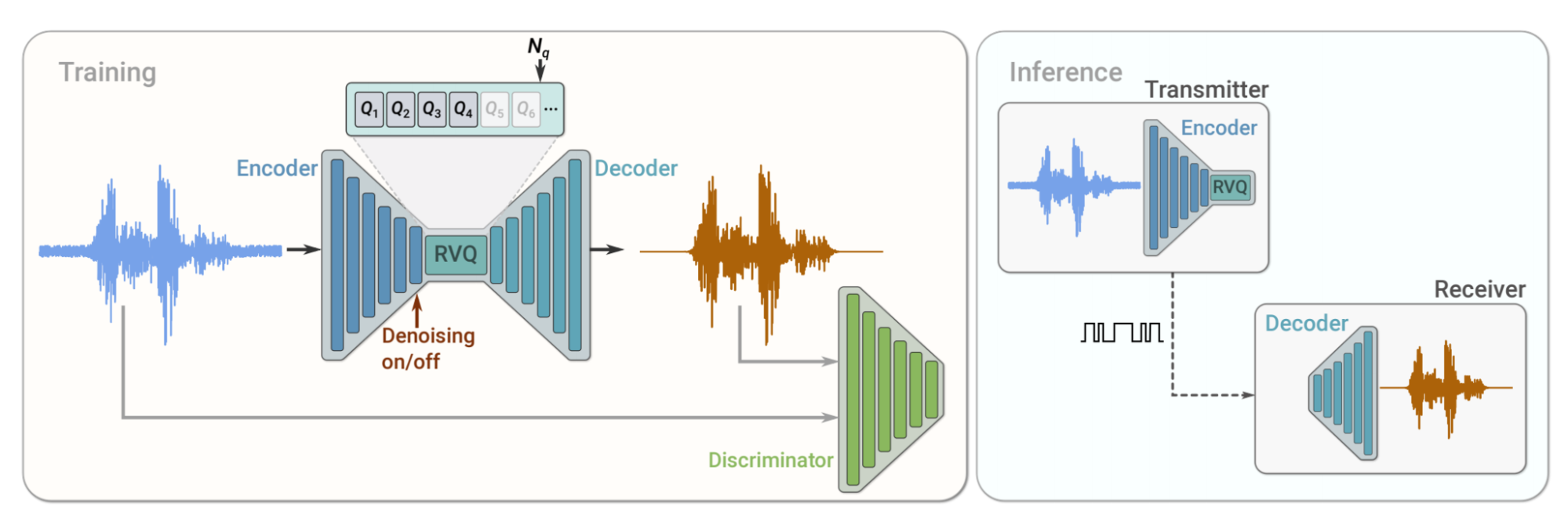
The main technical ingredient of SoundStream is a neural network, consisting of an encoder, decoder and quantizer, all of which are trained end-to-end. The encoder converts the input audio stream into a coded signal, which is compressed using the quantizer and then converted back to audio using the decoder. SoundStream leverages state-of-the-art solutions in the field of neural audio synthesis to deliver audio at high perceptual quality, by training a discriminator that computes a combination of adversarial and reconstruction loss functions that induce the reconstructed audio to sound like the uncompressed original input. Once trained, the encoder and decoder can be run on separate clients to efficiently transmit high-quality audio over a network.

SoundStream training and inference. During training, the encoder, quantizer and decoder parameters are optimized using a combination of reconstruction and adversarial losses, computed by a discriminator, which is trained to distinguish between the original input audio and the reconstructed audio. During inference, the encoder and quantizer on a transmitter client send the compressed bitstream to a receiver client that can then decode the audio signal.

Learning a Scalable Codec with Residual Vector Quantization
The encoder of SoundStream produces vectors that can take an indefinite number of values. In order to transmit them to the receiver using a limited number of bits, it is necessary to replace them by close vectors from a finite set (called a codebook), a process known as vector quantization. This approach works well at bitrates around 1 kbps or lower, but quickly reaches its limits when using higher bitrates. For example, even at a bitrate as low as 3 kbps, and assuming the encoder produces 100 vectors per second, one would need to store a codebook with more than 1 billion vectors, which is infeasible in practice.

In SoundStream, we address this issue by proposing a new residual vector quantizer (RVQ), consisting of several layers (up to 80 in our experiments). The first layer quantizes the code vectors with moderate resolution, and each of the following layers processes the residual error from the previous one. By splitting the quantization process in several layers, the codebook size can be reduced drastically. As an example, with 100 vectors per second at 3 kbps, and using 5 quantizer layers, the codebook size goes from 1 billion to 320. Moreover, we can easily increase or decrease the bitrate by adding or removing quantizer layers, respectively.

Because network conditions can vary while transmitting audio, ideally a codec should be “scalable” so that it can change its bitrate from low to high depending on the state of the network. While most traditional codecs are scalable, previous learnable codecs need to be trained and deployed specifically for each bitrate.

To circumvent this limitation, we leverage the fact that the number of quantization layers in SoundStream controls the bitrate, and propose a new method called “quantizer dropout”. During training, we randomly drop some quantization layers to simulate a varying bitrate. This pushes the decoder to perform well at any bitrate of the incoming audio stream, and thus helps SoundStream to become “scalable” so that a single trained model can operate at any bitrate, performing as well as models trained specifically for these bitrates.

Comparison of SoundStream models (higher is better) that are trained at 18 kbps with quantizer dropout (bitrate scalable), without quantizer dropout (not bitrate scalable) and evaluated with a variable number of quantizers, or trained and evaluated at a fixed bitrate (bitrate specific). The bitrate-scalable model (a single model for all bitrates) does not lose any quality when compared to bitrate-specific models (a different model for each bitrate), thanks to quantizer dropout.

A State-of-the-Art Audio Codec
SoundStream at 3 kbps outperforms Opus at 12 kbps and approaches the quality of EVS at 9.6 kbps, while using 3.2x–4x fewer bits. This means that encoding audio with SoundStream can provide a similar quality while using a significantly lower amount of bandwidth. Moreover, at the same bitrate, SoundStream outperforms the current version of Lyra, which is based on an autoregressive network. Unlike Lyra, which is already deployed and optimized for production usage, SoundStream is still at an experimental stage. In the future, Lyra will incorporate the components of SoundStream to provide both higher audio quality and reduced complexity.

SoundStream at 3kbps vs. state-of-the-art codecs. MUSHRA score is an indication of subjective quality (the higher the better).

The demonstration of SoundStream’s performance compared to Opus, EVS, and the original Lyra codec is presented in these audio examples, a selection of which are provided below.

Speech

Reference
Lyra (3kbps)
Opus (6kbps)
EVS (5.9kbps)
SoundStream (3kbps)  

Music

Reference
Lyra (3kbps)
Opus (6kbps)
EVS (5.9kbps)
SoundStream (3kbps)  

Joint Audio Compression and Enhancement
In traditional audio processing pipelines, compression and enhancement (the removal of background noise) are typically performed by different modules. For example, it is possible to apply an audio enhancement algorithm at the transmitter side, before audio is compressed, or at the receiver side, after audio is decoded. In such a setup, each processing step contributes to the end-to-end latency. Conversely, we design SoundStream in such a way that compression and enhancement can be carried out jointly by the same model, without increasing the overall latency. In the following examples, we show that it is possible to combine compression with background noise suppression, by activating and deactivating denoising dynamically (no denoising for 5 seconds, denoising for 5 seconds, no denoising for 5 seconds, etc.).

Original noisy audio  
Denoised output*
* Demonstrated by turning denoising on and off every 5 seconds.

Conclusion
Efficient compression is necessary whenever one needs to transmit audio, whether when streaming a video, or during a conference call. SoundStream is an important step towards improving machine learning-driven audio codecs. It outperforms state-of-the-art codecs, such as Opus and EVS, can enhance audio on demand, and requires deployment of only a single scalable model, rather than many.

SoundStream will be released as a part of the next, improved version of Lyra. By integrating SoundStream with Lyra, developers can leverage the existing Lyra APIs and tools for their work, providing both flexibility and better sound quality. We will also release it as a separate TensorFlow model for experimentation.

AcknowledgmentsThe work described here was authored by Neil Zeghidour, Alejandro Luebs, Ahmed Omran, Jan Skoglund and Marco Tagliasacchi. We are grateful for all discussions and feedback on this work that we received from our colleagues at Google.

Read More

Hooked on a Feeling: GFN Thursday Brings ‘NARAKA: BLADEPOINT’ to GeForce NOW

Calling all warriors. It’s a glorious week full of new games.

This GFN Thursday comes with the exciting release of the new battle royale NARAKA: BLADEPOINT, as well as the Hello Neighbor franchise as part of the 11 great games joining the GeForce NOW library this week.

Plus, the newest Assassin’s Creed Valhalla DLC has arrived on the cloud.

Real PC Games, Real PC Power

Gaming on GeForce NOW means having access to the real versions of PC games. And there are more than 1,000 PC titles streaming from the cloud, with more on the way every week. It also means being able to play these titles across devices like low-powered PCs, Macs, Chromebooks, SHIELD TVs or Android and iOS mobile devices with the power of the cloud.

Members can play new and exciting PC games like NARAKA:BLADEPOINT with the power of a gaming rig streaming to any GeForce NOW compatible device at GeForce-level performance.

Melee Meets Battle Royale

Only one can remain. The melee, combat battle royale NARAKA: BLADEPOINT is now available on Steam and can be streamed on GeForce NOW. It’ll also be available to stream from the Epic Games Store upon its release in September.

NARAKA: BLADEPOINT on GeForce NOW
How far will your grappling hook take you in the challenge on Morus Island?

Sixty players, heroes from around the world, will gather on Morus Island — and one will emerge victorious. Explore the vast, interactive world with a vertical design and experience unique gameplay powered by parkour and grappling hook movement. Learn to best use the brand-new resurrection system and unique character skills of a roster of characters with powerful abilities. And enjoy a vast arsenal of melee and ranged weapons along with the thrill of clashing blades and arrows flying in the battlefield.

Make your move. Press the assault on enemies with a grappling hook that can be aimed at anyone, anywhere and used to zip through obstacles to pounce on targets. Ambush opponents by hiding in the darkness and waiting for the right moment with deadly long-range takedowns or sneaky melee attacks. And avoid fights with a quick escape from less-favorable battles with a well-aimed grappling hook maneuver. Play your way to achieve victory.

NARAKA: BLADEPOINT on GeForce NOW
Become the ultimate warrior and crush your enemies in this new battle royale.

Thanks to the GeForce power of the cloud, gamers can battle with the best and all other online PC gamers playing awesome multiplayer games like NARAKA: BLADEPOINT.

“It’s great that GeForce NOW can introduce gamers playing on low-powered hardware to the stunning world of NARAKA,” said Ray Kuan, lead producer. “We love that more gamers will be able to enter the battlefield and enjoy the next generation of battle royale games in full PC glory across all of their devices.”

Become the last warrior standing and learn the truth of NARAKA’s world and its endless battles on GeForce NOW this week.

Hello, It’s the Games of the Week

This GFN Thursday is packed with 11 new titles available to stream on GeForce NOW, including the stealth horror franchise, Hello Neighbor.

Hello Neighbor on GeForce NOW
Find out what’s in the basement of your neighbor’s home in Hello Neighbor. Just don’t get caught.

What’s your neighbor hiding? Members can find out and play Hello Neighbor, a suspenseful story of sneaking into your neighbor’s house to figure out what horrible secrets he’s hiding in the basement. Don’t get too comfortable — The Neighbor will learn from your every move and leave nasty surprises for you.

And stream the dramatic prequel, Hello Neighbor: Hide and Seek, to follow the tragic story of the loss of a family member while playing a game of hide-and-seek that leads to the game that started it all.

The full list of awesome games joining the service this week includes:

Finally, members will be able to sack a famous city and play the glorious new Assassin’s Creed Valhalla: The Siege of Paris DLC upon release today on GeForce NOW.

While you plan your gaming escape this weekend, we’ve got an important question for you.

Some games are so gorgeous, they make us never want to leave.

If you had to spend your summer vacation in a game which one would it be? 🏖

🌩 NVIDIA GeForce NOW (@NVIDIAGFN) August 11, 2021

Tell us on Twitter or in the comments below, and we’ll catch up next week!

The post Hooked on a Feeling: GFN Thursday Brings ‘NARAKA: BLADEPOINT’ to GeForce NOW appeared first on The Official NVIDIA Blog.

Read More

Getting started with Amazon SageMaker Feature Store

In a machine learning (ML) journey, one crucial step before building any ML model is to transform your data and design features from your data so that your data can be machine-readable. This step is known as feature engineering. This can include one-hot encoding categorical variables, converting text values to vectorized representation, aggregating log data to a daily summary, and more. The quality of your features directly influences your model predictability, and often needs a few iterations until a model reaches an ideal level of accuracy. Data scientists and developers can easily spend 60% of their time designing and creating features, and the challenges go beyond writing and testing your feature engineering code. Features built at different times and by different teams aren’t consistent. Extensive and repetitive feature engineering work is often needed when productionizing new features. Difficulty tracking versions and up-to-date features aren’t easily accessible.

To address these challenges, Amazon SageMaker Feature Store provides a fully managed central repository for ML features, making it easy to securely store and retrieve features without the heavy lifting of managing the infrastructure. It lets you define groups of features, use batch ingestion and streaming ingestion, and retrieve the latest feature values with low latency.

For an introduction to Feature Store and a basic use case using a credit card transaction dataset for fraud detection, see New – Store, Discover, and Share Machine Learning Features with Amazon SageMaker Feature Store. For further exploration of its features, see Using streaming ingestion with Amazon SageMaker Feature Store to make ML-backed decisions in near-real time.

For this post, we focus on the integration of Feature Store with other Amazon SageMaker features to help you get started quickly. The associated sample notebook and the following video demonstrate how you can apply these concepts to the development of an ML model to predict the risk of heart failure.

The components of Feature Store

Feature Store is a centralized hub for features and associated metadata. Features are defined and stored in a collection called a feature group. You can visualize a feature group as a table in which each column is a feature, with a unique identifier for each row. In principle, a feature group is composed of features and values specific to each feature. A feature group’s definition is composed of a list of the following:

  • Feature definitions – These consist of a name and data types.
  • A record identifier name – Each feature group is defined with a record identifier name. It should be a unique ID to identify each instance of the data, for example, primary key, customer ID, transaction ID, and so on.
  • Configurations for its online and offline store – You can create an online or offline store. The online store is used for low-latency, real-time inference use cases, and the offline store is used for training and batch inference.

The following diagram shows how you can use Feature Store as part of your ML pipeline. First, you read in your raw data and transform it to features ready for exploration and modeling. Then you can create a feature store, configure it to an online or offline store, or both. Next you can ingest data via streaming to the online and offline store, or in batches directly to the offline store. After your feature store is set up, you can create a model using data from your offline store and access it for real time inference or batch inference.

For more hands-on experience, follow the notebook example for a step-by-step guide to build a feature store, train a model for fraud detection, and access the feature store for inference.

Export data from Data Wrangler to Feature Store

Because Feature Store can ingest data in batches, you can author features using Amazon SageMaker Data Wrangler, create feature groups in Feature Store, and ingest features in batches using a SageMaker Processing job with a notebook exported from Data Wrangler. This mode allows for batch ingestion into the offline store. It also supports ingestion into the online store if the feature group is configured for both online and offline use.

To start off, after you complete your data transformation steps and analysis, you can conveniently export your data preparation workflow into a notebook with one click. When you export your flow steps, you have the option of exporting your processing code to a notebook that pushes your processed features to Feature Store.

Choose Export step and Feature Store to automatically create your notebook. This notebook recreates the manual steps you created, creates a feature group, and adds features to an offline or online feature store, allowing you easily rerun your manual steps.

This notebook defines the schema instead of auto-detection of data types for each column of the data, with the following format:

column_schema = [
 { 
 "name": "Height", 
 "type": "long" 
 },
 { 
 "name": "Sum", 
 "type": "string" 
 }, 
 { 
 "name": "Time", 
 "type": "string"
  }
]

For more information on how to load the schema, map it, and add it as a FeatureDefinition that you can use to create the FeatureGroup, see Export to the SageMaker Feature Store.

Additionally, you must specify a record identifier name and event time feature name in the following code:

  • The record_identifier_name is the name of the feature whose value uniquely identifies a record defined in the feature store.
  • An EventTime is a point in time when a new event occurs that corresponds to the creation or update of a record in a feature. All records in the feature group must have a corresponding EventTime.

The notebook creates an offline store and the online by default with the following configuration set to True:

online_store_config = {
    "EnableOnlineStore": True
}

You can also disable an online store by setting EnableOnlineStore to False in the online and offline store configurations.

You can then run the notebook, and the notebook creates a feature group and processing job to process data in scale. The offline store is located in an Amazon Simple Storage Service (Amazon S3) bucket in your AWS account. Because Feature Store is integrated with Amazon SageMaker Studio, you can visualize the feature store by choosing Components and registries in the navigation pane, choosing Feature Store on the drop-down menu, and then finding your feature store on the list. You can check for feature definitions, manage feature group tags, and generate queries for the offline store.

Build a training set from an offline store

Now that you have created a feature store from your processed data, you can build a training dataset from your offline store by using services such as Amazon Athena, AWS Glue, or Amazon EMR. In the following example, because Feature Store automatically builds an AWS Glue Data Catalog when you create feature groups, you can easily create a training dataset with feature values from the feature group. This is done by utilizing the auto-built Data Catalog.

First, create an Athena query for your feature group with the following code. The table_name is the AWS Glue table that is automatically generated by Feature Store.

sample_query = your_feature_group.athena_query()
data_table = sample_query.table_name

You can then write your query using SQL on your feature group, and run the query with the .run() command and specify your S3 bucket location for the dataset to be saved there. You can modify the query to include any operations needed for your data like joining, filtering, ordering, and so on. You can further process the output DataFrame until it’s ready for modeling, then upload it to your S3 bucket so that your SageMaker trainer can directly read the input from the S3 bucket.

# define your Athena query
query_string = 'SELECT * FROM "'+data_table+'"'

# run Athena query. The output is loaded to a Pandas dataframe.
dataset = pd.DataFrame()
sample_query.run(query_string=query_string, output_location='s3://'+default_s3_bucket_name+'/query_results/')
sample_query.wait()
dataset = sample_query.as_dataframe()

Access your Feature Store for inference

After you build a model from the training set, you can access your online store conveniently to fetch a record and make predictions using the deployed model. Feature Store can be especially useful in supplementing data for inference requests because of the low-latency GetRecord functionality. In this example, you can use the following code to query the online feature group to build an inference request:

selected_id = str(194)

# Helper to parse the feature value from the record.

def get_feature_value(record, feature_name):
    return str(list(filter(lambda r: r['FeatureName'] == feature_name, record))[0]['ValueAsString'])

fs_response = featurestore_runtime.get_record(
                                               FeatureGroupName=your_feature_group_name,
                                               RecordIdentifierValueAsString=selected_id)
selected_record = fs_response['Record']
inference_request = [
    get_feature_value(selected_record, 'feature1'),
    get_feature_value(selected_record, 'feature2'),
    ....
    get_feature_value(selected_record, 'feature 10')
]

You can then call the deployed model predictor to generate a prediction for the selected record:

results = predictor.predict(','.join(inference_request), 
                            initial_args = {"ContentType": "text/csv"})
prediction = json.loads(results)

Integrate Feature Store in a SageMaker pipeline

Feature Store also integrates with Amazon SageMaker Pipelines to create, add feature search and discovery to, and reuse automated ML workflows. As a result, it’s easy to add feature search, discovery, and reuse to your ML workflow. The following code shows you how to configure the ProcessingOutput to directly write the output to your feature group instead of Amazon S3, so that you can maintain your model features in a feature store:

flow_step_outputs = []
flow_output = sagemaker.processing.ProcessingOutput(
    output_name=customers_output_name,
    feature_store_output=sagemaker.processing.FeatureStoreOutput(
        feature_group_name=your_feature_group_name), 
    app_managed=True)
flow_step_outputs.append(flow_output)

example_flow_step = ProcessingStep(
    name='SampleProcessingStep', 
    processor=flow_processor, # Your flow processor defined at the beginning of your pipeline
    inputs=flow_step_inputs, # Your processing and feature engineering steps, can be Data Wrangler flows
    outputs=flow_step_outputs)

Conclusion

In this post, we explored how Feature Store can be a powerful tool in your ML journey. You can easily export your data processing and feature engineering results to a feature group and build your feature store. After your feature store is all set up, you can explore and build training sets from your offline store, taking advantage of its integration with other AWS analytics services such as Athena, AWS Glue, and Amazon EMR. After you train and deploy a model, you can fetch records from your online store for real-time inference. Lastly, you can add a feature store as a part of a complete SageMaker pipeline in your ML workflow. Feature Store makes it easy to store and retrieve features as needed in ML development.

Give it a try, and let us know what you think!


About the Author

As a data scientist and consultant, Zoe Ma has helped bring the latest tools and technologies and data-driven insights to businesses and enterprises. In her free time, she loves painting and crafting and enjoys all water sports.

Courtney McKay is a consultant. She is passionate about helping customers drive measurable ROI with AI/ML tools and technologies. In her free time, she enjoys camping, hiking and gardening.

Read More

How Digitec Galaxus trains and serves millions of personalized newsletters per week with TFX

Posted by Christian Sager (Product Owner, Digitec Galaxus) and Anant Nawalgaria (ML Specialist, Google)

gif from blog titled how Digitec Galaxus trains and serves millions of personalized newsletters per week with TFX showing an animation of a cloud and people

In the retail industry it is important to be able to engage and excite users by serving personalized content on newsletters at scale. It is important to do this in a manner which leverages existing trends, while exploring and unearthing potentially new trends with an even higher user engagement. This project was done as a collaboration between Digitec Galaxus and Google, by designing a system based on Contextual Bandits to personalize newsletters for more than 2 million users every week.

To accomplish this, we leveraged several products in the TensorFlow ecosystem and Google Cloud including TF Agents, TensorFlow Extended (TFX) running on Vertex AI , to build a system that personalizes newsletters in a scalable, modularized and cost effective manner with low latency. In this article, we’ll highlight a few of the pieces, and point you to resources you can use to learn more.

About Digitec Galaxus

Digitec Galaxus AG is the largest online retailer in Switzerland. It offers a wide range of products to its customers, from electronics to clothes. As an online retailer, we naturally make use of recommendation systems, not only on our home or product pages but also in our newsletters. We have multiple recommendation systems in place already for newsletters, and have been extensive early adopters of the Google Cloud recommendations AI. Because we have multiple recommendation systems and very large amounts of data, we are faced with the following complications.

1. Personalization

We have over 12 recommenders that it uses in the newsletters, however we would like to contextualize these by choosing different recommenders (which in turn select the items) for different users. Furthermore, we would like to exploit existing trends as well as experiment with new ones.

2. Latency

We would like to ensure that the ranked list of recommenders can be retrieved with sub 50 ms latency.

3. End-to-end easy to maintain and generalizable/modular architecture

We wanted the solution to be architected using an easy to maintain, platform invariant, complete with all MLops capabilities required to train and use contextual bandits models. It was also important to us that it is built in a modular fashion such that it can be adapted easily to other use cases which have in mind such as recommendations on the homepage, Smartags and more.

Before we get to the details of how we built a machine learning infrastructure capable of dealing with all requirements, we’ll dig a little deeper into how we got here and what problem we’re trying to solve.

Using contextual bandits

Digitec Galaxus has multiple recommendation systems in place already. Because we have multiple recommendation systems, it is sometimes difficult to choose between them in a personalized fashion. Hence we reached out to Google seeking assistance with implementing Contextual Bandit driven recommendations, which personalizes our homepage as well as our newsletter. Because we only send newsletters to registered users, we can incorporate features for every user.

We chose TFAgents to implement the contextual bandit model. Training and serving pipelines were orchestrated by Vertex AI pipelines running TFX, which in turn used TFAgents for the development of the contextual bandit models. Here’s an overview of our approach.

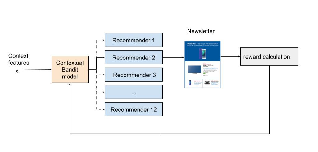
TFAgents to implement the contextual bandit model

Rewarding subscribes, and penalizing unsubscribes

Given some features (context) about the user, and each of the 12 available recommenders, we aim to suggest best recommender (action) which increases the chance (reward) of the user clicking (reward = 1) on at least one of the recommendations by the selected recommender, and minimizes the chance of incurring a click which leads to unsubscribe (reward = -1).

By formulating the problem and reward function in this manner, we hypothesized that the system would optimize for increasing clicks, while still showing relevant (and not click-baity) content to the user in order to sustain the potential increase in performance. This is because the reward functions penalizes an event when a user unsubscribes, which a click-baity content is likely to lead to. The problem was then tackled by using contextual bandits because of the fact that they excel at exploiting trends that work well, as well as exploring and uncovering potentially even better-performing trends.

Serving millions of users every week with low latency

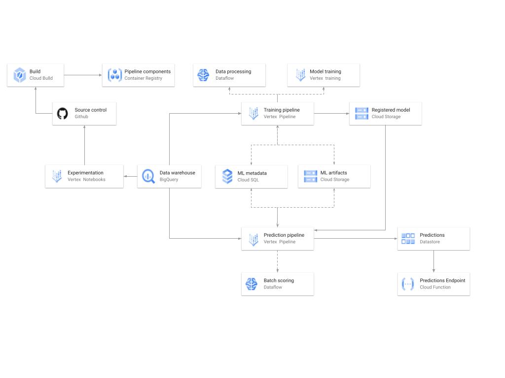
A diagram showing the high-level architecture of the recommendation training and prediction systems on GCP.

There’s a lot of detail here, as the architecture shown in the diagram covers three phases of ML development, training, and serving. Here are some of the key pieces.

Model development

Vertex Notebooks are used as data science environments for experimentation and prototyping, in addition to implementing model training and scoring components and pipelines. The source code is version controlled in GitHub. A continuous integration (CI) pipeline is set up to run unit tests, build pipeline components, and store the container images to Cloud Container Registry.

Training

The training pipeline is executed using TFX on Vertex Pipelines. In essence, the pipeline trains the model using new training data extracted from BigQuery, validates the produced model, and stores it in the model registry. In our system, the model registry is curated in Cloud Storage. The training pipeline uses Dataflow for large scale data extraction, validation, processing and model evaluation, as well as Vertex Training for large scale distributed training of the model. In addition, AI Platform Pipelines stores artifacts produced by the various pipeline steps to Cloud Storage, and information about these artifacts is stored in an ML metadata database in Cloud SQL.

Serving

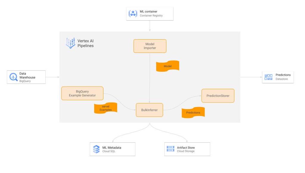
Predictions are produced using a batch prediction pipeline, and stored in Cloud Datastore for consumption. The batch prediction pipeline is made using TFX and runs on Vertex Pipelines. The pipeline uses the most recent model in the model registry to score the serving queries from BigQuery. A Cloud Function is provided as a REST/HTTP endpoint to retrieve predictions from Datastore.

Continuous Training Pipeline

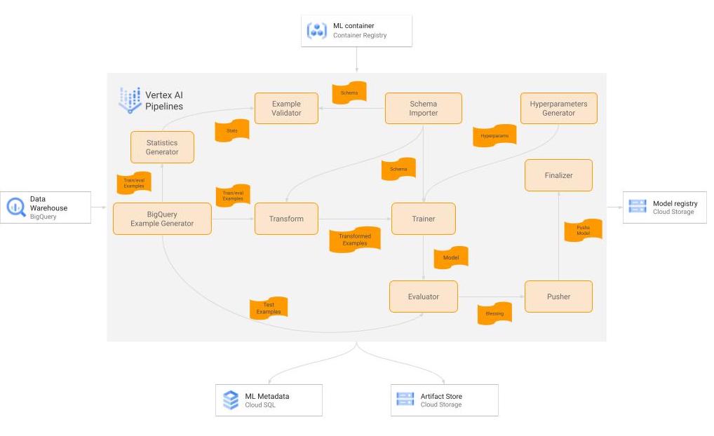
A diagram of the TFX pipeline for the training workflow.

There are many components used in our TFX-based Continuous training workflow, training is currently done on an on-demand basis, but later on it is planned to be executed on a bi-weekly cadence. Here is a little bit of detail on the important ones.

Raw Data

Our data consists of multiple datasets stored in heterogeneous formats across BigQuery tables and other formats, that are then joined in denormalized fashion by the customer into a single BigQuery table for training. To help avoid bias and drift in our model we train the model on a rolling window of 4 weeks cadence with one overlapping week per training cycle. This was a simple design choice as it was very straightforward to implement, as BigQuery has good compatibility as a source with TFX, and also allows the user to do some basic data preprocessing and cleaning during fetching.

BigQueryExampleGen

We first leverage BigQuery by leveraging built-in functions to preprocess the data. By embedding our own specific processes into the query calls made by the ExampleGen component, we were able to avoid building out a separate ETL that would exist outside the scope of a TFX pipeline. This ultimately proved to be a good way to get the model in production more quickly. This preprocessed data is then split into training and eval and converted to tf.Examples via the ExampleGen component.

Transform

This component does the necessary feature engineering and transformations necessary to handle strings, fill in missing values, log-normalize values, setup embeddings etc. The major benefit here is that the resulting transformation is ultimately prepended to the computational graph, so that the exact same code is used for training and serving. The Transform component runs on Cloud Dataflow in production.

Trainer

The Trainer component trains the model using TF-Agents. We leverage parallel training on Vertex Training to speed things up. The model is designed such that the user id passes in from the input to the output unaltered, so that it can be used as part of the downstream serving pipeline. The Trainer component runs on Vertex Training in production.

Evaluator

The Evaluator compares the existing production model to the model received by the Trainer and prepares the metrics required by the validator component to bless the “better” one for use in production. The model gating criteria is based on the AUC scores as well as counterfactual policy evaluation and possibly other metrics in the future. It is easy to implement custom metrics which meet the business requirements owing to the extensibility of the evaluator component. The Evaluator runs on Vertex AI.

Pusher

The Pusher’s primary function is to send the blessed model to our TFServing deployment for production. However, we added functionality to use the custom metrics produced in the Evaluator to determine decisioning criteria to be used in serving, and attach that to the computational graph. The level of abstraction available in TFX components made it easy to make this custom modification. Overall, the modification allows the pipeline to operate without a human in the loop so that we are able to make model updates frequently, while continuing to deliver consistent performance on metrics that are important to our business.

HyperparametersGen

This is a custom TFX component which creates a dictionary with hyperparameters (e.g., batch size, learning rate) and stores the dictionary as an artifact. The hyperparameters are passed as input to the trainer.

ServingModelResolver

This custom component takes a serving policy (which includes exploration) and a corresponding eval policy (without exploration), and resolves which policy will be used for serving.

Pushing_finalizer

This custom component copies the pushed/blessed model from the TFX artifacts directory to a curated destination.

The out-of-box components from TFX provided most of the functionality we require, and it is easy to create some new custom components to make the entire pipeline satisfy our requirements. There are also other components of the pipeline such as StatisticsGen (which also runs on Dataflow).

Batch Prediction Pipeline

A diagram showing the TFX pipeline for the batch prediction workflow.

Here are a few of the key pieces of our batch prediction system.

Inference Dataset

Our inference dataset has nearly identical format to the training dataset, except that it is emptied and repopulated with new data daily.

BigQueryExampleGen

Just like for the Training pipeline, we use this component to read data from BigQuery and convert it into tf.Examples.

Model Importer

This component imports the computation graph exported by the Pusher component of the training pipeline. As mentioned above, since it contains the whole computation graph generated by the training pipeline, including feature transformation and the tf.Agents model (including the exploration/exploitation aspect), this is very portable and prevents train/test skew.

BulkInferrer

As the name implies, this component uses the imported computation graph to perform mass inference on the inference dataset. It runs on Cloud Dataflow in production and makes it very easy to scale.

PredictionStorer

This is a custom Python Component which takes the inference results from Bulkinfererrer, post-processes them to format/filter the fields as required, and persists it to Cloud Datastore. This runs on Cloud Dataflow in production as well.

Serving is done via cloud functions which take the user ids as input, and returns the precomputed results for each userId stored in DataStore with sub 50 ms latency.

Extending the work so far

In the few months since implementation of the first version we have been making dozens of improvements to the pipeline, everything from changing the architecture/approach of the original model, to changing the way the model’s results are used in the downstream application to generate newsletters. Moreover, each of these improvements brings new value to us more quickly than we’ve been able to in the past.

Since our initial implementation of this reference architecture, we have released a simple Vertex AI pipeline based github code samples to implementing recommender systems using TF Agents here. By using this template and guide, it will help them build recommender systems using contextual bandits on GCP in a scalable, modularized, low latency and cost effective manner. It’s quite remarkable how many of the existing TFX components that we have in place carry over to new projects, and even more so how drastically we’ve reduced the time it takes to get a model in production. As a result, even the software engineers on our team without much ML expertise feel confident in being able to reuse this architecture and adapt it to more use cases. The data scientists are able to spend more of their time optimizing the parameters and architectures of the models they produce, understanding their impact on the business, and ultimately delivering more value to the users and the business.

Acknowledgements

None of this would have been possible without the joint collaboration of the following Googlers: Khalid Salama, Efi Kokiopoulou, Gábor Bartók and Digitec Galaxus’s team of engineers.

A Google Cloud blog on this project can be found here.

Read More

Run ML inference on AWS Snowball Edge with Amazon SageMaker Edge Manager and AWS IoT Greengrass

You can use AWS Snowball Edge devices in locations like cruise ships, oil rigs, and factory floors with limited to no network connectivity for a wide range of machine learning (ML) applications such as surveillance, facial recognition, and industrial inspection. However, given the remote and disconnected nature of these devices, deploying and managing ML models at the edge is often difficult. With AWS IoT Greengrass and Amazon SageMaker Edge Manager, you can perform ML inference on locally generated data on Snowball Edge devices using cloud-trained ML models. You not only benefit from the low latency and cost savings of running local inference, but also reduce the time and effort required to get ML models to production. You can do all this while continuously monitoring and improving model quality across your Snowball Edge device fleet.

In this post, we talk about how you can use AWS IoT Greengrass version 2.0 or higher and Edge Manager to optimize, secure, monitor, and maintain a simple TensorFlow classification model to classify shipping containers (connex) and people.

Getting started

To get started, order a Snowball Edge device (for more information, see Creating an AWS Snowball Edge Job). You can order a Snowball Edge device with an AWS IoT Greengrass validated AMI on it.

After you receive the device, you can use AWS OpsHub for Snow Family or the Snowball Edge client to unlock the device. You can start an Amazon Elastic Compute Cloud (Amazon EC2) instance with the latest AWS IoT Greengrass installed or use the commands on AWS OpsHub for Snow Family.

Launch and install an AMI with the following requirements, or provide an AMI reference on the Snowball console before ordering and it will be shipped with all libraries and data in the AMI:

  • The ML framework of your choice, such as TensorFlow, PyTorch, or MXNet
  • Docker (if you intend to use it)
  • AWS IoT Greengrass
  • Any other libraries you may need

Prepare the AMI at the time of ordering the Snowball Edge device on AWS Snow Family console. For instructions, see Using Amazon EC2 Compute Instances. You also have the option to update the AMI after Snowball is deployed to your edge location.

Install the latest AWS IoT Greengrass on Snowball Edge

To install AWS IoT Greengrass on your device, complete the following steps:

  1. Install the latest AWS IoT Greengrass on your Snowball Edge device. Make sure dev_tools=True is set to have ggv2 cli See the following code:
sudo -E java -Droot="/greengrass/v2" -Dlog.store=FILE  -jar ./MyGreengrassCore/lib/Greengrass.jar  --aws-region region  --thing-name MyGreengrassCore  --thing-group-name MyGreengrassCoreGroup  --tes-role-name GreengrassV2TokenExchangeRole  --tes-role-alias-name GreengrassCoreTokenExchangeRoleAlias  --component-default-user ggc_user:ggc_group  --provision true  --setup-system-service true  --deploy-dev-tools true

We reference the --thing-name you chose here when we set up Edge Manager.

  1. Run the following command to test your installation:
aws greegrassv2 help
  1. On the AWS IoT console, validate the successfully registered Snowball Edge device with your AWS IoT Greengrass account.

Optimize ML models with Edge Manager

We use Edge Manger to deploy and manage the model on Snowball Edge.

  1. Install the Edge Manager agent on Snowball Edge using the latest AWS IoT Greengrass.
  2. Train and store your ML model.

You can train your ML model using any framework of your choice and save it to an Amazon Simple Storage Service (Amazon S3) bucket. In the following screenshot, we use TensorFlow to train a multi-label model to classify connex and people in an image. The model used here is saved to an S3 bucket by first creating a .tar file.

After the model is saved (TensorFlow Lite in this case), you can start an Amazon SageMaker Neo compilation job of the model and optimize the ML model for Snowball Edge Compute (SBE_C).

  1. On the SageMaker console, under Inference in the navigation pane, choose Compilation jobs.
  2. Choose Create compilation job.

  1. Give your job a name and create or use an existing role.

 If you’re creating a new AWS Identity and Access Management (IAM) role, ensure that SageMaker has access to the bucket in which the model is saved.

  1. In the Input configuration section, for Location of model artifacts, enter the path to model.tar.gz where you saved the file (in this case, s3://feidemo/tfconnexmodel/connexmodel.tar.gz).
  2. For Data input configuration, enter the ML model’s input layer (its name and its shape). In this case, it’s called keras_layer_input and its shape is [1,224,224,3], so we enter {“keras_layer_input”:[1,224,224,3]}.

  1. For Machine learning framework, choose TFLite.

  1. For Target device, choose sbe_c.
  2. Leave Compiler options
  3. For S3 Output location, enter the same location as where your model is saved with the prefix (folder) output. For example, we enter s3://feidemo/tfconnexmodel/output.

  1. Choose Submit to start the compilation job.

Now you create a model deployment package to be used by Edge Manager.

  1. On the SageMaker console, under Edge Manager, choose Edge packaging jobs.
  2. Choose Create Edge packaging job.
  3. In the Job properties section, enter the job details.
  4. In the Model source section, for Compilation job name, enter the name you provided for the Neo compilation job.
  5. Choose Next.

  1. In the Output configuration section, for S3 bucket URI, enter where you want to store the package in Amazon S3.
  2. For Component name, enter a name for your AWS IoT Greengrass component.

This step creates an AWS IoT Greengrass model component where the model is downloaded from Amazon S3 and uncompressed to local storage on Snowball Edge.

  1. Create a device fleet to manage a group of devices, in this case, just one (SBE).
  2. For IAM role¸ enter the role generated by AWS IoT Greengrass earlier (–tes-role-name).

Make sure it has the required permissions by going to IAM console, searching for the role, and adding the required policies to it.

  1. Register the Snowball Edge device to the fleet you created.

  1. In the Device source section, enter the device name. The IoT name needs to match the name you used earlier—in this case, –thing-name MyGreengrassCore.

You can register additional Snowball devices on the SageMaker console to add them to the device fleet, which allows you to group and manage these devices together.

Deploy ML models to Snowball Edge using AWS IoT Greengrass

In the previous sections, you unlocked and configured your Snowball Edge device. The ML model is now compiled and optimized for performance on Snowball Edge. An Edge Manager package is created with the compiled model and the Snowball device is registered to a fleet. In this section, you look at the steps involved in deploying the ML model for inference to Snowball Edge with the latest AWS IoT Greengrass.

Components

AWS IoT Greengrass allows you to deploy to edge devices as a combination of components and associated artifacts. Components are JSON documents that contain the metadata, the lifecycle, what to deploy when, and what to install. Components also define what operating system to use and what artifacts to use when running on different OS options.

Artifacts

Artifacts can be code files, models, or container images. For example, a component can be defined to install a pandas Python library and run a code file that will transform the data, or to install a TensorFlow library and run the model for inference. The following are example artifacts needed for an inference application deployment:

  • gRPC proto and Python stubs (this can be different based on your model and framework)
  • Python code to load the model and perform inference

These two items are uploaded to an S3 bucket.

Deploy the components

The deployment needs the following components:

  • Edge Manager agent (available in public components at GA)
  • Model
  • Application

Complete the following steps to deploy the components:

  1. On the AWS IoT console, under Greengrass, choose Components, and create the application component.
  2. Find the Edge Manager agent component in the public components list and deploy it.
  3. Deploy a model component created by Edge Manager, which is used as a dependency in the application component.
  4. Deploy the application component to the edge device by going to the list of AWS IoT Greengrass deployments and creating a new deployment.

If you have an existing deployment, you can revise it to add the application component.

Now you can test your component.

  1. In your prediction or inference code deployed with application component, code in the logic to access files locally on the Snowball Edge device (for example, in the incoming folder) and have the predictions or processed files be moved to a processed folder.
  2. Log in to the device to see if the predictions have been made.
  3. Set up the code to run on a loop, checking the incoming folder for new files, processing the files, and moving them to the processed folder.

The following screenshot is an example setup of files before deployment inside the Snowball Edge.

After deployment, all the test images have classes of interest and therefore are moved to the processed folder.

Clean up

To clean up everything or reimplement this solution from scratch, stop all the EC2 instances by invoking the TerminateInstance API against EC2-compatible endpoints running on your Snowball Edge device. To return your Snowball Edge device, see Powering Off the Snowball Edge and Returning the Snowball Edge Device.

Conclusion

This post walked you through how to order a Snowball Edge device with an AMI of your choice. You then compile a model for the edge using SageMaker, package that model using Edge Manager, and create and run components with artifacts to perform ML inference on Snowball Edge using the latest AWS IoT Greengrass. With Edge Manager, you can deploy and update your ML models on a fleet of Snowball Edge devices, and monitor performance at the edge with saved input and prediction data on Amazon S3. You can also run these components as long-running AWS Lambda functions that can spin up a model and wait for data to do inference.

You combine several features of AWS IoT Greengrass to create an MQTT client and use a pub/sub model to invoke other services or microservices. The possibilities are endless.

By running ML inference on Snowball Edge with Edge Manager and AWS IoT Greengrass, you can optimize, secure, monitor, and maintain ML models on fleets of Snowball Edge devices. Thanks for reading and please do not hesitate to leave questions or comments in the comments section.

To learn more about AWS Snow Family, AWS IoT Greengrass, and Edge Manager, check out the following:


About the Authors

Raj Kadiyala is an AI/ML Tech Business Development Manager in AWS WWPS Partner Organization. Raj has over 12 years of experience in Machine Learning and likes to spend his free time exploring machine learning for practical every day solutions and staying active in the great outdoors of Colorado.


Nida Beig is a Sr. Product Manager – Tech at Amazon Web Services where she works on the AWS Snow Family team. She is passionate about understanding customer needs, and using technology as a conductor of transformative thinking to deliver consumer products. Besides work, she enjoys traveling, hiking, and running.

Read More

Q&A with Georgia Tech’s Amy Bruckman, research award recipient in online content governance

In this monthly interview series, we turn the spotlight on members of the academic community and the important research they do — as thought partners, collaborators, and independent contributors.

For August, we nominated Amy Bruckman, a professor at Georgia Tech. Bruckman is a winner of the 2019 Content Governance RFP, which sought proposals that helped expand research and advocacy work in the area of online content governance. In this Q&A, Bruckman shares more about her area of specialization, her winning research proposal, and her upcoming book. She also shares what inspires her in her academic work.

Q: Tell us about your role at Georgia Tech and the type of research you specialize in.

Amy Bruckman: I am professor and senior associate chair in the School of Interactive Computing at Georgia Tech. We are halfway between an I-school and a CS department — more technical than most I-schools and more interdisciplinary than most CS departments.

I founded my first online community in 1993, and I am endlessly fascinated by how the design features of an online environment shape human behavior. My students and I build new tools to support novel kinds of online interaction, and we also study existing systems using a mixed-methods approach. My specialty is qualitative methods. My students and I participate online and take field notes on what we observe (methods inspired by sociology and anthropology), and we also interview people about their experiences (building on clinical interview techniques from psychology). I partner with people who do big data and NLP research, and I’ve found that qualitative and quantitative methods are usually more powerful when used together.

Q: What have you been working on lately?

AB: Personally, lately I’ve been focused on my book Should You Believe Wikipedia? Online Communities and the Construction of Knowledge. It is coming out in January from Cambridge University Press. In the book, I try to explain how online communities are designed, with a particular focus on how people can collaboratively build knowledge.

Q: You were a winner of the 2019 Content Governance RFP. What was your winning proposal about?

AB: Our research asks the question, What happens after a controversial figure who regularly breaks platform rules is kicked off, or “deplatformed”? In particular, we studied what happened after Alex Jones, Milo Yiannopoulos, and Owen Benjamin were kicked off Twitter.

Q: What were the results of this research?

AB: My coauthors (Shagun Jhaver, Christian Boylston, and Diyi Yang) and I found that deplatforming significantly reduced the number of conversations about those individuals. More important, the overall activity and toxicity levels of supporters declined after deplatforming. For example, Milo encouraged his followers to attack actress Leslie Jones. After he was deplatformed, his supporters were better behaved. The full paper will appear at CSCW 2021.

Q: What inspires you in your academic work?

AB: I believe that our field is at a crossroads: The internet needs some redesign to support healthy communities and a working public sphere. The last chapter of my book is focused on how we can help the internet to bring out the best in us all. I try to work toward that goal in my research and in my teaching. Every fall, I teach our required ethics class “Computing, Society, and Professionalism,” and in spring, I teach “Design of Online Communities.” It’s a privilege to teach students about these issues, and the students have impact as they go on to design and build the information systems we all use every day.

Q: Where can people learn more about you and your work?

AB: My book Should You Believe Wikipedia? will be published in early 2022, and there is a sample chapter on my website.

The post Q&A with Georgia Tech’s Amy Bruckman, research award recipient in online content governance appeared first on Facebook Research.

Read More

Registration now open for the 2021 Instagram Workshop on Recommendation Systems at Scale

Instagram invites the academic community and industry peers to join the first Instagram Workshop on Recommendation Systems at Scale, taking place virtually on Thursday, September 23. Those interested may register at the link below.

Register

Production recommendation systems in large social and commerce platforms introduce complex and unprecedented challenges. The goal of this workshop is to bring together leading researchers and practitioners in related fields to share knowledge and explore research collaboration opportunities between academia and industry.

“Every day, we help over a billion people connect with their friends, interests, businesses, and creators they love on Instagram. To ensure that a community of this size finds new and inspiring content, we need to constantly evolve our recommendation systems technology. Collaborating with like-minded industry and academic experts allows us to do just that,” says Aameek Singh, Engineering Director, Instagram.

Confirmed speakers

Below is the list of confirmed speakers as of today.

  • Anoop Deoras (AWS, Amazon)
  • Diane Hu (Etsy)
  • Jonathan J Hunt (Twitter Cortex Applied Research)
  • Chris Wiggins (The New York Times)

As speakers are confirmed, they will be added to the registration page, along with their full bios and topics. View additional event details and register to attend at the link below.

Register

The post Registration now open for the 2021 Instagram Workshop on Recommendation Systems at Scale appeared first on Facebook Research.

Read More