“Lift as you lead”: Meet 2 women defining responsible AI

At Google, Marian Croak’s technical research team, The Center for Responsible AI and Human-Centered Technology, and Jen Gennai’s operations and governance team, Responsible Innovation, collaborate often on creating a fairer future for AI systems.

The teams complement each other to support computer scientists, UX researchers and designers, product managers and subject matter experts in the social sciences, human rights and civil rights. Collectively, their teams include more than 200 people around the globe focused on putting our AI Principles – Google’s ethical charter – into practice.

“The intersection of AI systems and society is a critical area of my team’s technical research,” Marian says. “Our approach includes working directly with people who use and are impacted by AI systems. Working together with Jen’s central operations team, the idea is to make AI more useful and reduce potential harm before products launch.”

For Women’s History Month, we wanted to talk to them both about this incredibly meaningful work and how they bring their lived experiences to it.

How do you define “responsible AI”?

Marian: It’s the technical realization of our AI Principles. We need to understand how AI systems are performing in respect to fairness, transparency, interpretability, robustness and privacy. When gaps occur, we fix them. We benchmark and evaluate how product teams are adopting what Jen and I call smart practices. These are trusted practices based on patterns we see across Google as we’re developing new AI applications, and the data-driven results of applying these practices over time.

Jen: There are enormous opportunities to use AI for positive impact — and the potential for harm, too. The key is ethical deployment. “Responsible AI” for me means taking deliberate steps to ensure technology works the way it’s intended to and doesn’t lead to malicious or unintended negative consequences. This involves applying the smart practices Marian mentioned through repeatable processes and a governance structure for accountability.

How do your teams work together?

Marian: They work hand in hand. My team conducts scientific research and creates open source tools like Fairness Indicators and Know Your Data. A large portion of our technical research and product work is centered in societal context and human and civil rights, so Jen’s team is integral to understanding the problems we seek to help solve.

Jen: The team I lead defines Google policies, handles day-to-day operations and central governance structure, and conducts ethical assessments. We’re made up of user researchers, social scientists, ethicists, human rights specialists, policy and privacy advisors and legal experts.

One team can’t work without the other! This complementary relationship allows many different perspectives and lived experiences to inform product design decisions. Here’s an example, which was led by women from a variety of global backgrounds: Marian’s team designed a streamlined, open source format for documenting technical details of datasets, called data cards. When researchers on the Translate team, led by product manager Romina Stella, recently developed a new dataset for studying and preventing gender bias in machine learning, members of my team, Anne P., N’Mah Y. and Reena Jana, reviewed the dataset for alignment with the AI Principles. They recommended that the Translate researchers publish a data card for details on how the dataset was created and tested. The Translate team then worked with UX designer Mahima Pushkarna on Marian’s team to create and launch the card alongside the dataset.

I’m inspired most when someone tells me I can’t do something. No matter what obstacles you face, believe you have the skills, the knowledge and the passion to make your dreams come true.

How did you end up working in this very new field?

Marian: I’ve always been drawn to hard problems. This is a very challenging area! It’s so multifaceted and constantly evolving. That excites me. It’s an honor to work with so many passionate people who care so deeply about our world and understanding how to use technology for social good.

I’ll always continue to seek out solutions to these problems because I understand the profound impact this work will have on our society and our world, especially communities underrepresented in the tech industry.

Jen: I spent many years leading User Research and User Advocacy on Google’s Trust and Safety team. An area I focused on was ML Fairness. I never thought I’d get to work on it full time. But in 2016 my leadership team wanted to have a company-wide group concentrating on worldwide positive social benefits of AI. In 2017, I joined the team that was writing and publishing the AI Principles. Today, I apply my operational knowledge to make sure that as a company, we meet the obligations we laid out in the Principles.

What advice do you have for girls and women interested in pursuing careers in responsible tech?

Marian: I’m inspired most when someone tells me I can’t do something. No matter what obstacles you face, believe you have the skills, the knowledge and the passion to make your dreams come true. Find motivation in the small moments, find motivation in those who doubt you, but most importantly, never forget to believe in the greatness of you.

Jen: Don’t limit yourself even if you don’t have a computer science degree. I don’t. I was convinced I’d work in sustainability and environmental non-profits, and now I lead a team working to make advanced technologies work better for everyone. This space requires so many different skills, whether in program management, policy, engineering, UX or business and strategy.

My mantra is “lift as you lead.” Don’t just build a network for yourself; build a supportive network to empower everyone who works with you — and those who come after you, especially those who are currently underrepresented in the tech sector. Your collective presence in this space makes a positive impact! And it’s even stronger when you build a better future together.

Read More

Automated, scalable, and cost-effective ML on AWS: Detecting invasive Australian tree ferns in Hawaiian forests

This is blog post is co-written by Theresa Cabrera Menard, an Applied Scientist/Geographic Information Systems Specialist at The Nature Conservancy (TNC) in Hawaii.

In recent years, Amazon and AWS have developed a series of sustainability initiatives with the overall goal of helping preserve the natural environment. As part of these efforts, AWS Professional Services establishes partnerships with organizations such as The Nature Conservancy (TNC), offering financial support and consulting services towards environmental preservation efforts. The advent of big data technologies is rapidly scaling up ecological data collection, while machine learning (ML) techniques are increasingly utilized in ecological data analysis. AWS is in a unique position to help with data storage and ingestion as well as with data analysis.

Hawaiian forests are essential as a source of clean water and for preservation of traditional cultural practices. However, they face critical threats from deforestation, species extinction, and displacement of native species by invasive plants. The state of Hawaii spends about half a billion dollars yearly fighting invasive species. TNC is helping to address the invasive plant problem through initiatives such as the Hawaii Challenge, which allows anyone with a computer and internet access to participate in tagging invasive weeds across the landscape. AWS has partnered with TNC to build upon these efforts and develop a scalable, cloud-based solution that automates and expedites the detection and localization of invasive ferns.

Among the most aggressive species invading the Hawaiian forests is the Australian tree fern, originally introduced as an ornamental, but now rapidly spreading across several islands by producing numerous spores that are easily transported by the wind. The Australian tree fern is fast growing and outcompetes other plants, smothering the canopy and affecting several native species, resulting in a loss of biological diversity.

Currently, detection of the ferns is accomplished by capturing images from fixed wing aircraft surveying the forest canopy. The imagery is manually inspected by human labelers. This process takes significant effort and time, potentially delaying the mitigation efforts by ground crews by weeks or longer. One of the advantages of utilizing a computer vision (CV) algorithm is the potential time savings because the inference time is expected to take only a few hours.

Machine learning pipeline

The following diagram shows the overall ML workflow of this project. The first goal of the AWS-TNC partnership was to automate the detection of ferns from aerial imagery. A second goal was to evaluate the potential of CV algorithms to reliably classify ferns as either native or invasive. The CV model inference can then form the basis of a fully automated AWS Cloud-native solution that enhances the capacity of TNC to efficiently and in a timely manner detect invasive ferns and direct resources to highly affected areas. The following diagram illustrates this architecture.

In the following sections, we cover the following topics:

  • The data processing and analysis tools utilized.
  • The fern detection model pipeline, including training and evaluation.
  • How native and invasive ferns are classified.
  • The benefits TNC experienced through this implementation.

Data processing and analysis

Aerial footage is acquired by TNC contractors by flying fixed winged aircraft above affected areas within the Hawaiian Islands. Heavy and persistent cloud cover prevents use of satellite imagery. The data available to TNC and AWS consists of raw images and metadata allowing the geographical localization of the inferred ferns.

Images and geographical coordinates

Images received from aerial surveys are in the range of 100,000 x 100,000 pixels and are stored in the JPEG2000 (JP2) format, which incorporates geolocation and other metadata. Each pixel can be associated to specific Universal Transverse Mercator (UTM) geospatial coordinates. The UTM coordinate system divides the world into north-south zones, each 6 degrees of longitude wide. The first UTM coordinate (northing) refers to the distance between a geographical position and the equator, measured with the north as the positive direction. The second coordinated (easting) measures the distance, in meters, towards east, starting from a central meridian that is uniquely assigned for each zone. By convention, the central meridian in each region has a value of 500,000, and a meter east of the region central meridian therefore has the value 500,001. To convert between pixel coordinates and UTM coordinates, we utilize the affine transform as outlined in the following equation, where x’, y’ are UTM coordinates and x, y are pixel coordinates. The parameters a, b, c, d, e, and f of the affine transform are provided as part of the JP2 file metadata.

For the purposes of labeling, training and inference of the raw JP2 files are divided into non-overlapping 512 x 512-pixel JPG files. The extraction of smaller sub-images from the original JP2 necessitates the creation of an individual affine transform directly from each individual extracted JPG file. These operations were performed utilizing the rasterio and affine Python packages with AWS Batch and facilitated the reporting of the position of inferred ferns in UTM coordinates.

Data labeling

Visual identification of ferns in the aerial images is complicated by several factors. Most of the information is aggregated in the green channel, and there is a high density of foliage with frequent partial occlusion of ferns by both nearby ferns and other vegetation. The information of interest to TNC is the relative density of ferns per acre, therefore it’s important to count each individual fern even in the presence of occlusion. Given these goals and constraints, we chose to utilize an object detection CV framework.

To label the data, we set up an Amazon SageMaker Ground Truth  labeling job. Each bounding box was intended to be centered in the center of the fern, and to cover most of the fern branches, while at the same time attempting to minimize the inclusion of other vegetation. The labeling was performed by the authors following consultation with TNC domain experts. The initial labeled dataset included 500 images, each typically containing several ferns, as shown in the following example images. In this initial labeled set we did not distinguish between native and invasive ferns.

Fern Object detection model training and update

In this section we discuss training the initial fern detection model, data labeling in Ground Truth and the model update through retraining. We also discuss using Amazon Augmented AI (Amazon A2I) for the model update, and using AWS Step Functions for the overall fern detection inference pipeline.

Initial fern detection model training

We utilized the Amazon SageMaker object detection algorithm because it provides state-of-the-art performance and can be easily integrated with other SageMaker services such as Ground Truth, endpoints, and Batch Transform jobs. We utilized the Single Shot MultiBox Detector (SSD) framework and base network vgg-16. This network comes pre-trained on millions of images and thousands of classes from the ImageNet dataset. We break all the given TNC JP2 images into 512 x 512-pixel tiles as the training dataset. There are about 5,000 small JPG images, and we randomly selected 4,500 images as the training dataset and 500 images as the validation dataset. After hyperparameter tuning, we chose the following hyperparameters for the model training: class=1, overlap_threshold=0.3, learning_rate=0.001, and epochs=50. The initial model’s mean average precision (mAP) computed on the validation set  is 0.49. After checking the detection results and TNC labels, we discovered that many ferns that were detected as ferns by our object detection model were not labeled as ferns from TNC fern labels, as shown in the following images.

Therefore, we decided to use Ground Truth to relabel a subset of the fern dataset in the attempt to improve model performance and then compare ML inference results with this initial model to check which approach is better.

Data labeling in Ground Truth

To label the fern dataset, we set up a Ground Truth job of 500 randomly selected 512 x 512-pixel images. Each bounding box was intended to be centered in the center of the fern, and to cover most of the fern branches, while at the same time attempting to minimize the inclusion of other vegetation. The labeling was performed by AWS data scientists following consultation with TNC domain experts. In this labeled dataset, we didn’t distinguish between native and invasive ferns.

Retraining the fern detection model

The first model training iteration utilized a set of 500 labeled images, of which 400 were in the training set and 100 in the validation set. This model achieved a mAP (computed on the validation set) score of 0.46, which isn’t very high. We next used this initial model to produce predictions on a larger set of 3,888 JPG images extracted from the available JP2 data. With this larger image set for training, the model achieved a mAP score of 0.87. This marked improvement (as shown in the following example images) illustrates the value of automated labeling and model iteration.

Based on these findings we determined that Ground Truth labeling plus automated labeling and model iteration appear to significantly increase prediction performance. To further quantify the performance of the resulting model, a set of 300 images were randomly selected for an additional round of validation. We found that when utilizing a threshold of 0.3 for detection confidence, 84% of the images were deemed by the labeler to have the correct number of predicted ferns, with 6.3% being overcounts and 9.7% being undercounts. In most cases, the over/undercounting was off by only one or two ferns out of five or six present in an image, and is therefore not expected to significantly affect the overall estimation of fern density per acre.

Amazon A2I for fern detection model update

One challenge for this project is that the images coming in every year are taken from aircraft, so the altitude, angles, and light condition of the images may be different. The model trained on the previous dataset needs to be retrained to maintain good performance, but labeling ferns for a new dataset is labor-intensive. Therefore, we used Amazon A2I to integrate human review to ensure accuracy with new data. We used 360 images as a test dataset; 35 images were sent back to for review because these images didn’t have predictions with a confidence score over 0.3. We relabeled these 35 images and retrained the model using incremental learning in Amazon A2I. The retrained model showed significant improvement from the previous model on many aspects, such as detections under darker light conditions, as shown in the following images. These improvements made the new model perform fairly well on new dataset with very few human reviews and relabeling work.

Fern detection inference pipeline

The overall goal of the TNC-AWS partnership is the creation of an automated pipeline that takes as input the JP2 files and produces as output UTM coordinates of the predicted ferns. There are three main tasks:

  • The first is the ingestion of the large JP2 file and its division into smaller 512 x 512 JPG files. Each of these has an associated affine transform that can generate UTM coordinates from the pixel coordinates.
  • The second task is the actual inference and detection of potential ferns and their locations.
  • The final task assembles the inference results into a single CSV file that is delivered to TNC.

The orchestration of the pipeline was implemented using Step Functions. As is the case for the inference, this choice automates many of the aspects of provisioning and releasing computing resources on an as-needed basis. Additionally, the pipeline architecture can be visually inspected, which enhances dissemination to the customer. Finally, as updated models potentially become available in the future, they can be swapped in with little or no disruption to the workflow. The following diagram illustrates this workflow.

When the inference pipeline was used in batch mode on a source image of 10,000 x 10,000 pixels, and allocating an m4.large instance to SageMaker batch transform, the whole inference workflow ran within 25 minutes. Of these, 10 minutes was taken by the batch transform, and the rest by Step Functions steps and AWS Lambda functions. TNC expects sets up to 24 JP2 images at one time, about twice a year. By adjusting the size and number of instances to be used by the batch transform, we expect that the inference pipeline can be fully run within 24 hours.

Fern classification

In this section, we discuss how we applied the SageMaker Principal Component Analysis (PCA) algorithm to the bounding boxes and validated the classification results.

Application of PCA to fern bounding boxes

To determine whether it is possible to distinguish between the Australian tree fern and native ferns without the substantial effort of labeling a large set of images, we implemented an unsupervised image analysis procedure. For each predicted fern, we extracted the region inside the bounding box and saved it as a separate image. Next, these images were embedded in a high dimensional vector space by utilizing the img2vec approach. This procedure generated a 2048-long vector for each input image. These vectors were analyzed by utilizing Principal Component Analysis as implemented in the SageMaker PCA algorithm. We retained for further analysis the top three components, which together accounted for more than 85% of the variance in the vector data.

For each of the top three components, we extracted the associated images with the highest and lowest scores along the component. These images were visually inspected by AWS data scientists and TNC domain experts, with the goal of identifying whether the highest and lowest scores are associated with native or invasive ferns. We further quantified the classification power of each principal component by manually labeling a small set of 100 fern images as either invasive or native and utilizing the scikit-learn utility to obtain metrics such as area under the precision-recall curve for each of the three PCA components. When the PCA scores were used as inputs to a binary classifier (see the following graph), we found that PCA2 was the most discriminative, followed by PCA3, with PCA1 displaying only modest performance in distinguishing between native and invasive ferns.

Validation of classification results

We then examined images with the biggest and smallest PCA2 values with TNC domain experts to check if the algorithm can differentiate native and invasive ferns effectively. After going over 100 sample fern images, TNC experts determined that the images with the smallest PCA2 values are very likely to be native ferns, and the images with the largest PCA2 values are very likely to be invasive ferns (see the following example images). We would like to further investigate this approach with TNC in the near future.

Conclusion

The major benefits to TNC from adopting the inference pipeline proposed in this post are twofold. First, substantial cost savings is achieved by replacing months-long efforts by human labelers with an automatic pipeline that incurs minimal inference costs. Although exact costs can depend on several factors, we estimate the cost reductions to be at least of an order of magnitude. The second benefit is the reduction of time from data collection to the initiation of mitigation efforts. Currently, manual labeling for a dozen large JP2 files take several weeks to complete, whereas the inference pipeline is expected to take a matter of hours, depending on the number and size of inference instances allocated. A faster turnaround time would impact the capacity of TNC to plan routes for the crews responsible for treating the invasive ferns in a timely manner, and potentially find appropriate treatment windows considering the seasonality and weather patterns on the islands.

To get started using Ground Truth, see Build a highly accurate training dataset with Amazon SageMaker Ground Truth. Also learn more about Amazon ML by going to the Amazon SageMaker product page, and explore visual workflows for modern applications by going to the AWS Step Functions product page.


About the Authors

Dan Iancu is a data scientist with AWS. He has joined AWS three years ago and has worked with a variety of customers including in Health Care and Life Sciences, the space industry and the public sector. He believes in the importance of bringing value to the customer as well as contributing to environmental preservation by utilizing ML tools.

Kara Yang is a Data Scientist in AWS Professional Services. She is passionate about helping customers achieve their business goals with AWS cloud services. She has helped organizations build ML solutions across multiple industries such as manufacturing, automotive, environmental sustainability and aerospace.

Arkajyoti Misra is a Data Scientist at Amazon LastMile Transportation. He is passionate about applying Computer Vision techniques to solve problems that helps the earth. He loves to work with non-profit organizations and is a founding member of ekipi.org.

Annalyn Ng is a Senior Solutions Architect based in Singapore, where she designs and builds cloud solutions for public sector agencies. Annalyn graduated from the University of Cambridge, and blogs about machine learning at algobeans.com. Her book, Numsense! Data Science for the Layman, has been translated into multiple languages and is used in top universities as reference text.

Theresa Cabrera Menard is an Applied Scientist/Geographic Information Systems Specialist at The Nature Conservancy (TNC) in Hawai`i, where she manages a large dataset of high-resolution imagery from across the Hawaiian Islands.  She was previously involved with the Hawai`i Challenge that used armchair conservationists to tag imagery for weeds in the forests of Kaua`i.

Veronika Megler is a Principal Consultant, Big Data, Analytics & Data Science, for AWS Professional Services. She holds a PhD in Computer Science, with a focus on spatio-temporal data search. She specializes in technology adoption, helping customers use new technologies to solve new problems and to solve old problems more efficiently and effectively.

Read More

Automatically generate model evaluation metrics using SageMaker Autopilot Model Quality Reports

Amazon SageMaker Autopilot helps you complete an end-to-end machine learning (ML) workflow by automating the steps of feature engineering, training, tuning, and deploying an ML model for inference. You provide SageMaker Autopilot with a tabular data set and a target attribute to predict. Then, SageMaker Autopilot automatically explores your data, trains, tunes, ranks and finds the best model. Finally, you can deploy this model to production for inference with one click.

What’s new?

The newly launched feature, SageMaker Autopilot Model Quality Reports, now reports your model’s metrics to provide better visibility into your model’s performance for regression and classification problems. You can leverage these metrics to gather more insights about the best model in the Model leaderboard.

These metrics and reports that are available in a new “Performance” tab under the “Model details” of the best model include confusion matrices, an area under the receiver operating characteristic (AUC-ROC) curve and an area under the precision-recall curve (AUC-PR). These metrics help you understand the false positives/false negatives (FPs/FNs), tradeoffs between true positives (TPs) and false positives (FPs), as well as the tradeoffs between precision and recall to assess the best model performance characteristics.

Running the SageMaker Autopilot experiment

The Data Set

We use UCI’s bank marketing data set to demonstrate SageMaker Autopilot Model Quality Reports. This data contains customer attributes, such as age, job type, marital status, and others that we’ll use to predict if the customer will open an account with the bank. The data set refers to this account as a term deposit. This makes our case a binary classification problem – the prediction will either be “yes” or “no”. SageMaker Autopilot will generate several models on our behalf to best predict potential customers. Then, we’ll examine the Model Quality Report for SageMaker Autopilot’s best model.

Prerequisites

To initiate a SageMaker Autopilot experiment, you must first place your data in an Amazon Simple Storage Service (Amazon S3) bucket. Specify the bucket and prefix that you want to use for training. Make sure that the bucket is in the same Region as the SageMaker Autopilot experiment. You must also make sure that the Identity and Access Management (IAM) role Autopilot has permissions to access the data in Amazon S3.

Creating the experiment

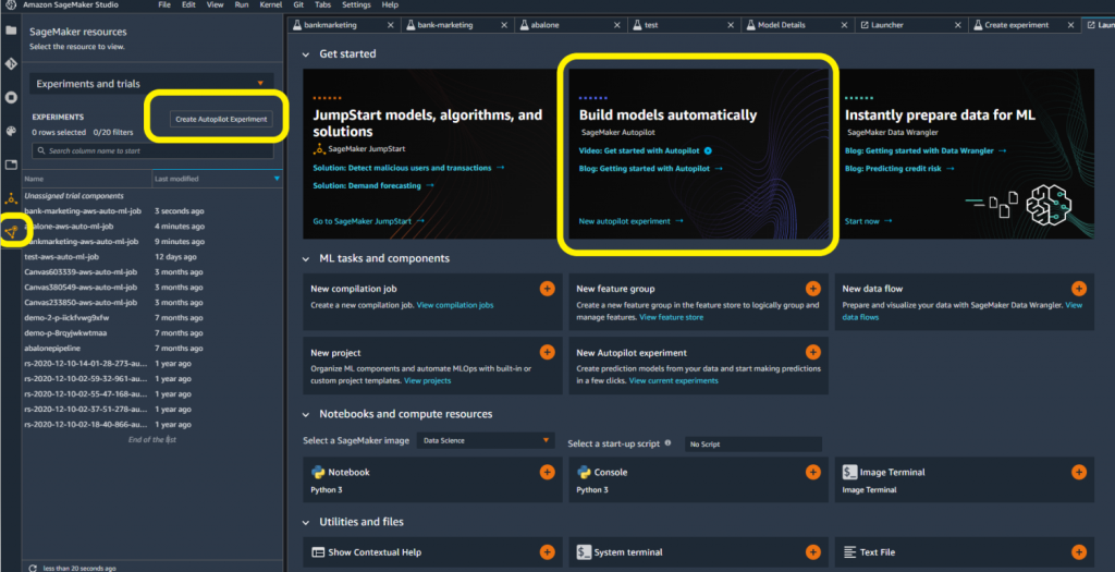
You have several options for creating a SageMaker Autopilot experiment in SageMaker Studio. By opening a new launcher, you may be able to access SageMaker Autopilot directly. If not, then you can select the SageMaker resources icon on the left-hand side. Next, you can select Experiments and trials from the drop-down menu.

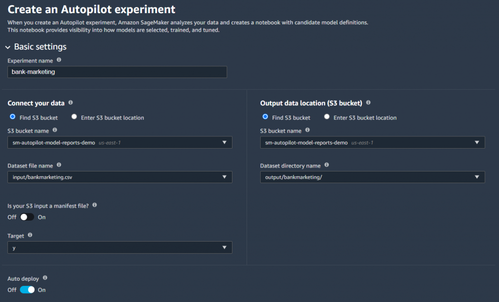
  1. Give your experiment a name.
  2. Connect to your data source by selecting the Amazon S3 bucket and file name.
  3. Choose the output data location in Amazon S3.
  4. Select the target column for your data set. In this case, we’re targeting the “y” column to indicate yes/no.
  5. Optionally, provide an endpoint name if you wish to have SageMaker Autopilot automatically deploy a model endpoint.
  6. Leave all of the other advanced settings as default, and select Create Experiment.

Once the experiment completes, you can see the results in SageMaker Studio. SageMaker Autopilot will present the best model among the different models that it trains. You can view details and results for different trials, but we’ll use the best model to demonstrate the use of Model Quality Reports.

  1. Select the model, and right-click to Open in model details.
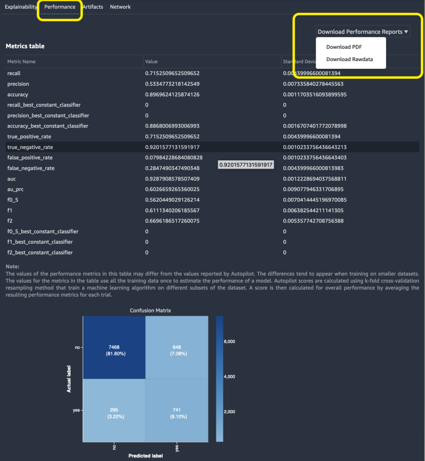
  2. Within the model details, select the Performance tab. This shows model metrics through visualizations and plots.
  3. Under Performance, select Download Performance Reports as PDF.

Interpreting the SageMaker Autopilot Model Quality Report

The Model Quality Report summarizes the SageMaker Autopilot job and model details. We’ll focus on the report’s PDF format, but you can also access the results as JSON. Because SageMaker Autopilot determined our data set as a binary classification problem, SageMaker Autopilot aimed to maximize the F1 quality metric to find the best model. SageMaker Autopilot chooses this by default. However, there is flexibility to choose other objective metrics, such as accuracy and AUC. Our model’s F1 score is 0.61. To interpret an F1 score, it helps to first understand a confusion matrix, which is explained by the Model Quality Report in the outputted PDF.

Confusion Matrix

A confusion matrix helps to visualize model performance by comparing different classes and labels. The SageMaker Autopilot experiment created a confusion matrix that shows the actual labels as rows, and the predicated labels as columns in the Model Quality Report. The upper-left box shows customers that didn’t open an account with the bank that were correctly predicted as ‘no’ by the model. These are true negatives (TN). The lower-right box shows customers that did open an account with the bank that were correctly predicted as ‘yes’ by the model. These are true positives (TP).

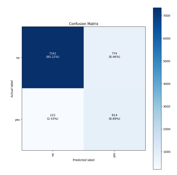
The bottom-left corner shows the number of false negatives (FN). The model predicted that the customer wouldn’t open an account, but the customer did. The upper-right corner shows the number of false positives (FP). The model predicted that the customer would open an account, but the customer did not actually do so.

Model Quality Report Metrics

The Model Quality Report explains how to calculate the false positive rate (FPR) and the true positive rate (TPR).

Recall or False Positive Rate (FPR) measures the proportion of actual negatives that were falsely predicted as opening an account (positives). The range is 0 to 1, and a smaller value indicates a better predictive accuracy.

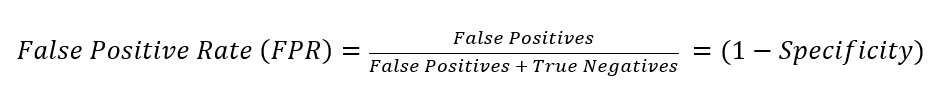
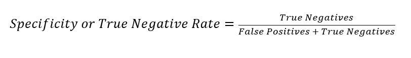
Note that the FPR is also expressed as 1-Specificity, where Specificity or True Negative Rate (TNR) is the proportion of the TNs correctly identified as not opening an account (negatives).

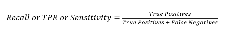
Recall/Sensitivity/True Positive Rate (TPR) measures the fraction of actual positives that were predicted as opening an account. The range is also 0 to 1, and a larger value indicates a better predictive accuracy. This is also known as Recall/Sensitivity. This measure expresses the ability to find all of the relevant instances in a dataset.

Precision measures the fraction of actual positives that were predicted as positives out of all of those predicted as positive. The range is 0 to 1, and a larger value indicates better accuracy. Precision expresses the proportion of the data points that our model says was relevant and that were actually relevant. Precision is a good measure to consider, especially when the costs of FP is high – for example with email spam detection.

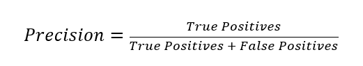
Our model shows a precision of 0.53 and a recall of 0.72.

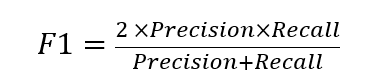
F1 Score demonstrates our target metric, which is the harmonic mean of precision and recall. Because our data set is imbalanced in favor of many ‘no’ predictions, F1 takes both FP and FN into account to give the same weight to precision and recall.

The report explains how to interpret these metrics. This can help if you’re unfamiliar with these terms. In our example, precision and recall are important metrics for a binary classification problem, as they’re used to calculate the F1 score. The report explains that an F1 score can vary between 0 and 1. The best possible performance will score 1, whereas 0 will indicate the worst. Remember that our model’s F1 score is 0.61.

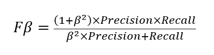
Fβ Score is the weighted harmonic mean of precision and recall. Moreover, the F1 score is the same as Fβ with β=1. The report provides the Fβ Score of the classifier, where β takes 0.5, 1, and 2.

Metrics Table

Depending on the problem, you may find that SageMaker Autopilot maximizes another metric, such as accuracy, for a multi-class classification problem. Regardless of the problem type, Model Quality Reports produce a table that summarizes your model’s metrics available both inline and in the PDF report. You can learn more about the metric table in the documentation.

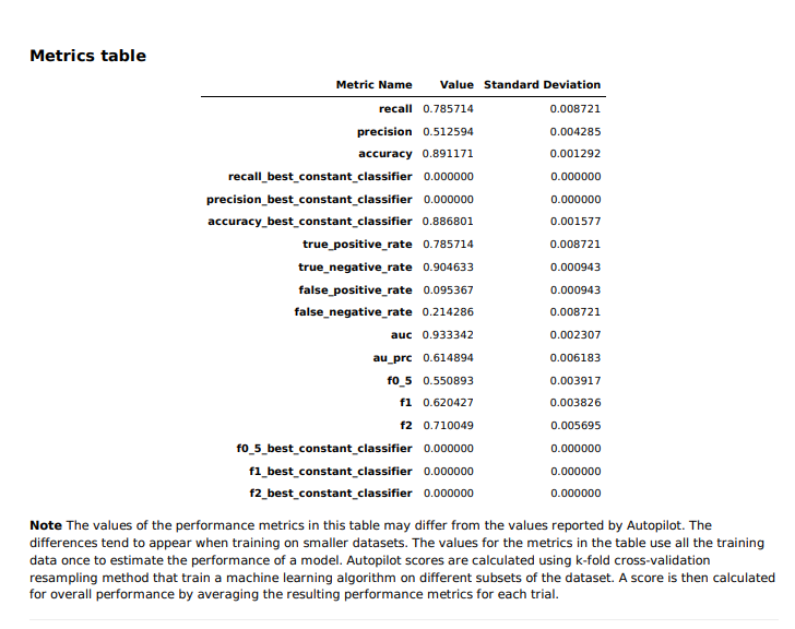
The best constant classifier – a classifier that serves as a simple baseline to compare against other more complex classifiers – always predicts a constant majority label that is provided by the user. In our case, a ‘constant’ model would predict ‘no’, since that is the most frequent class and considered to be a negative label. The metrics for the trained classifier models (such as f1, f2, or recall) can be compared to those for the constant classifier, i.e., the baseline. This makes sure that the trained model performs better than the constant classifier. Fβ scores (f0_5, f1, and f2, where β takes the values of 0.5, 1, and 2 respectively) are the weighted harmonic mean of precision and recall. This reaches its optimal value at 1 and its worst value at 0.

In our case, the best constant classifier always predicts ‘no’. Therefore, accuracy is high at 0.89, but the recall, precision, and Fβ scores are 0. If the dataset is perfectly balanced where there is no single majority or minority class, we would have seen much more interesting possibilities for the precision, recall, and Fβ scores of the constant classifier.

Furthermore, you can view these results in JSON format as shown in the following sample. Υou can access both the PDF and JSON files through the UI, as well as Amazon SageMaker Python SDK using the S3OutputPath element in OutputDataConfig structure in the CreateAutoMLJob/DescribeAutoMLJob API response.

{
  "version" : 0.0,
  "dataset" : {
    "item_count" : 9152,
    "evaluation_time" : "2022-03-16T20:49:18.661Z"
  },
  "binary_classification_metrics" : {
    "confusion_matrix" : {
      "no" : {
        "no" : 7468,
        "yes" : 648
      },
      "yes" : {
        "no" : 295,
        "yes" : 741
      }
    },
    "recall" : {
      "value" : 0.7152509652509652,
      "standard_deviation" : 0.00439996600081394
    },
    "precision" : {
      "value" : 0.5334773218142549,
      "standard_deviation" : 0.007335840278445563
    },
    "accuracy" : {
      "value" : 0.8969624125874126,
      "standard_deviation" : 0.0011703516093899595
    },
    "recall_best_constant_classifier" : {
      "value" : 0.0,
      "standard_deviation" : 0.0
    },
    "precision_best_constant_classifier" : {
      "value" : 0.0,
      "standard_deviation" : 0.0
    },
    "accuracy_best_constant_classifier" : {
      "value" : 0.8868006993006993,
      "standard_deviation" : 0.0016707401772078998
    },
    "true_positive_rate" : {
      "value" : 0.7152509652509652,
      "standard_deviation" : 0.00439996600081394
    },
    "true_negative_rate" : {
      "value" : 0.9201577131591917,
      "standard_deviation" : 0.0010233756436643213
    },
    "false_positive_rate" : {
      "value" : 0.07984228684080828,
      "standard_deviation" : 0.0010233756436643403
    },
    "false_negative_rate" : {
      "value" : 0.2847490347490348,
      "standard_deviation" : 0.004399966000813983
    },
………………….

ROC and AUC

Depending on the problem type, you may have varying thresholds for what’s acceptable as an FPR. For example, if you’re trying to predict if a customer will open an account, then it may be more acceptable to the business to have a higher FP rate. It can be riskier to miss extending offers to customers who were incorrectly predicted ‘no’, as opposed to offering customers who were incorrectly predicted ‘yes’. Changing these thresholds to produce different FPRs requires you to create new confusion matrices.

Classification algorithms return continuous values known as prediction probabilities. These probabilities must be transformed into a binary value (for binary classification). In binary classification problems, a threshold (or decision threshold) is a value that dichotomizes the probabilities to a simple binary decision. For normalized projected probabilities in the range of 0 to 1, the threshold is set to 0.5 by default.

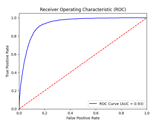
For binary classification models, a useful evaluation metric is the area under the Receiver Operating Characteristic (ROC) curve. The Model Quality Report includes a ROC graph with the TP rate as the y-axis and the FPR as the x-axis. The area under the receiver operating characteristic (AUC-ROC) represents the trade-off between the TPRs and FPRs.

You create a ROC curve by taking a binary classification predictor, which uses a threshold value, and assigning labels with prediction probabilities. As you vary the threshold for a model, you cover from the two extremes. When the TPR and the FPR are both 0, it implies that everything is labeled “no”, and when both the TPR and FPR are 1 it implies that everything is labeled “yes”.

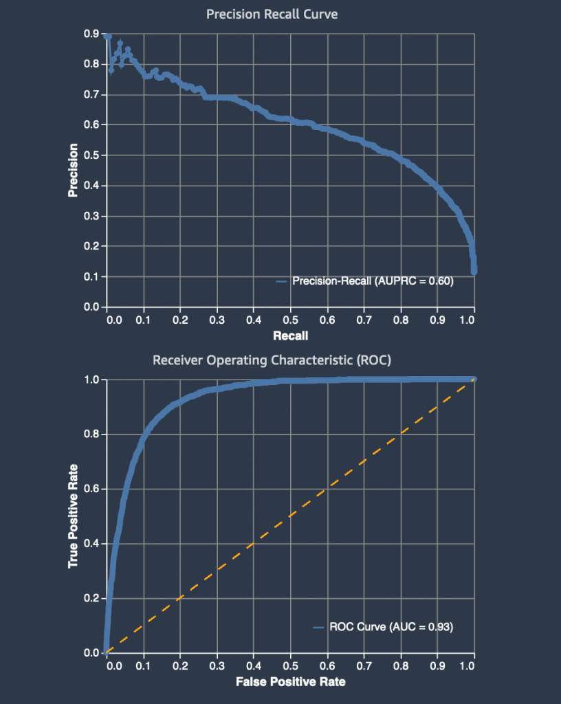
A random predictor that labels “Yes” half of the time and “No” the other half of the time would have a ROC that’s a straight diagonal line (red-dotted line). This line cuts the unit square into two equally-sized triangles. Therefore, the area under the curve is 0.5. An AUC-ROC value of 0.5 would mean that your predictor was no better at discriminating between the two classes than randomly guessing whether a customer would open an account or not. The closer the AUC-ROC value is to 1.0, the better its predictions are. A value below 0.5 indicates that we could actually make our model produce better predictions by reversing the answer that it gives us. For our best model, the AUC is 0.93.

Precision Recall Curve

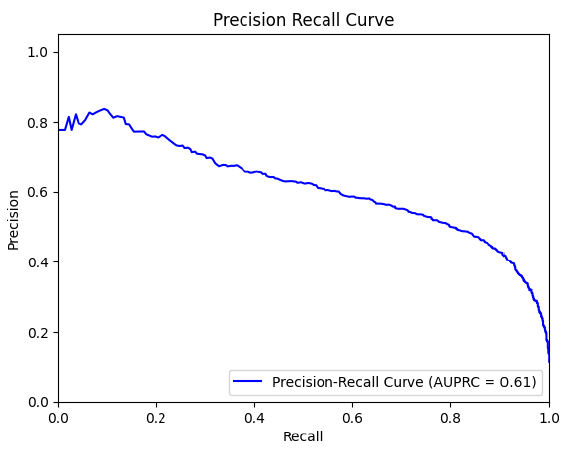
The Model Quality Report also created a Precision Recall (PR) Curve to plot the precision (y-axis) and the recall (x-axis) for different thresholds – much like the ROC curve. PR Curves, often used in Information Retrieval, are an alternative to ROC curves for classification problems with a large skew in the class distribution.

For these class imbalanced datasets, PR Curves especially become useful when the minority positive class is more interesting than the majority negative class. Remember that our model shows a precision of 0.53 and a recall of 0.72. Furthermore, remember that the best constant classifier can’t discriminate between ‘yes’ and ‘no’. It would predict a random class or a constant class every time.

The curve for a balanced dataset between ‘yes’ and ‘no’ would be a horizontal line at 0.5, and thus would have an area under the PR curve (AUPRC) as 0.5. To create the PRC, we plot various models on the curve at varying thresholds, in the same way as the ROC curve. For our data, the AUPRC is 0.61.

Model Quality Report Output

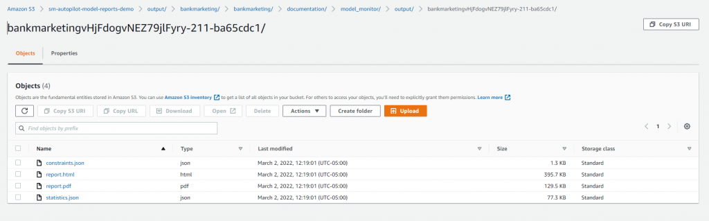
You can find the Model Quality Report in the Amazon S3 bucket that you specified when designating the output path before running the SageMaker AutoPilot experiment. You’ll find the reports under the documentation/model_monitor/output/<autopilot model name>/ prefix saved as a PDF.

Conclusion

SageMaker Autopilot Model Quality Reports makes it easy for you to quickly see and share the results of a SageMaker Autopilot experiment. You can easily complete model training and tuning using SageMaker Autopilot, and then reference the generated reports to interpret the results. Whether you end up using SageMaker Autopilot’s best model, or another candidate, these results can be a helpful starting point to evaluating a preliminary model training and tuning job. SageMaker Autopilot Model Quality Reports helps reduce the time needed to write code and produce visuals for performance evaluation and comparison.

You can easily incorporate autoML into your business cases today without having to build a data science team. SageMaker documentation provides numerous samples to help you get started.


About the Authors

Peter Chung is a Solutions Architect for AWS, and is passionate about helping customers uncover insights from their data. He has been building solutions to help organizations make data-driven decisions in both the public and private sectors. He holds all AWS certifications as well as two GCP certifications. He enjoys coffee, cooking, staying active, and spending time with his family.

Arunprasath Shankar is an Artificial Intelligence and Machine Learning (AI/ML) Specialist Solutions Architect with AWS, helping global customers scale their AI solutions effectively and efficiently in the cloud. In his spare time, Arun enjoys watching sci-fi movies and listening to classical music.

Ali Takbiri is an AI/ML specialist Solutions Architect, and helps customers by using Machine Learning to solve their business challenges on the AWS Cloud.

Pradeep Reddy is a Senior Product Manager in the SageMaker Low/No Code ML team, which includes SageMaker Autopilot, SageMaker Automatic Model Tuner. Outside of work, Pradeep enjoys reading, running and geeking out with palm sized computers like raspberry pi, and other home automation tech.

Read More

Teens Develop Handwriting-Recognition AI for Detecting Parkinson’s Disease

When Tanish Tyagi published his first research paper a year ago on deep learning to detect dementia, it started a family-driven pursuit.

Great-grandparents in his family had suffered from Parkinson’s, a genetic disease that affects more than 10 million people worldwide. So the now 16-year-old turned to that next, together with his sister, Riya, 14.

The siblings, from Short Hills, New Jersey, published a research paper in the fall about using machine learning to detect Parkinson’s disease by focusing on micrographia, a handwriting disorder that’s a marker for Parkinson’s.

They aim to make a model widely accessible so that early detection is possible for people around the world with limited access to clinics.

“Can we make some real change, can we not only impact our own family, but also see what’s out there and explore what we can do about something that might be a part of our lives in the future?” said Riya.

The Tyagis, who did the research over their summer break, attend prestigious U.S. boarding school Phillips Exeter Academy, alma mater to Mark Zuckerberg, Nobel Prize winners and one U.S. president.

When they aren’t busy with school or extracurricular research, they might be found pitching their STEM skills-focused board game (pictured above), available to purchase through Kickstarter.

Spotting Micrographia for Signs

Tanish decided to pursue research on Parkinson’s in February 2021, when he was just 15. He had recently learned about micrographia, a handwriting disorder that is a common symptom of Parkinson’s.

Micrographia in handwriting shows up as small text and exhibits tremors, involuntary muscle contractions and slow movement in the hands.

Not long after, Tanish heard a talk by Penn State University researchers Ming Wang and Lijun Zhang on Parkinson’s. So he sought their guidance on pursuing it for detection, and they agreed to supervise the project. Wang is also working with labs at Massachusetts General Hospital in connection with this research.

“Tanish and Riya’s work aims to enhance prediction of Micrographia by performing secondary analysis of public handwriting images and adopting state-of-art machine learning methods. The findings could help patients receive early diagnosis and treatment for better healthcare outcomes”, said Dr. Zhang, Associate Professor from Institute for Personalized Medicine at Penn State University.

In their paper, the Tyagis used NVIDIA GPU-driven machine learning for feature extraction of micrographia characteristics. Their dataset included open-source images of drawing exams from 53 healthy people and 105 Parkinson’s patients. They extracted several features from these images that allowed them to analyze tremors in writing.

“These are features that we had identified from different papers, and that we saw others had had success with,” said Riya.

With a larger and more balanced dataset, their high prediction accuracy of about 93 percent could get even better, said Tanish.

Developing a CNN for Diagnosis

Tanish had previously used his lab’s NVIDIA GeForce RTX 3080 GPU on a natural language processing project for dementia research. But neither sibling had much experience with computer vision before they began the Parkinson’s project.

Currently, the two are working on a convolutional neural network with transfer learning to put together a model that could be helpful for real-time diagnosis, said Riya.

“We’re working on processing the image from a user by feeding it into the model and then returning comprehensive results so that the user can really understand the diagnosis that the model is making,” Tanish said.

But first the Tyagis said they would like to increase the size of their dataset to improve the model’s accuracy. Their aim is to develop the model further and build a website. They want Parkinson’s detection to be so easy that people can fill out a handwriting assessment form and submit it for detection.

“It could be deployed to the general public and used in clinical settings, and that would be just amazing,” said Tanish.

The post Teens Develop Handwriting-Recognition AI for Detecting Parkinson’s Disease appeared first on NVIDIA Blog.

Read More

Go with the flow state: What music and AI have in common

Carrie Cai, Ben Zevenbergen and Johnny Soraker all work on developing artificial intelligence (AI) responsibly at Google, in the larger research community and across the technology industry. Carrie is a research scientist focusing on human-AI interaction, Ben is an ethicist and policy advisor and Johnny is an AI Principles ethicist. They all work within a global team of experts from a variety of fields, including the social sciences and humanities, focused on the ethical development of AI. They’re driven to make systems that are fair, inclusive and focused on people.

But they have more than their work in common: They’re all accomplished musicians who’ve studied music, composed and published pieces and even played at the professional level. We wanted to know more about their musical backgrounds, and how this creative interest informs their work building AI systems that take everyone into account.

What instrument — or instruments — do you play?

Ben: Guitar, bass and drums.

Johnny: Mainly drums these days, but I’ve also done ambient and electronica.

Carrie: I play piano and I also compose music.

Where did your interest in playing music come from?

Ben: I grew up in a musical family where instruments were always lying around. My parents’ friends would bring their instruments when they came to visit and our house would turn into a music venue. I enrolled in a music degree in my late teens to become a professional drummer. Then, a year later, I serendipitously became a bassist: I went to law school in the Netherlands, and the university band already had someone who was a better drummer than I was — but they needed a bassist, so I grabbed the opportunity.

Carrie: I started out in the Yamaha music program when I was six, where rather than learning technical piano playing skills you focus on ear training, hearing the music and how to play as an ensemble. I think that foundation led me to be a lot more creative with my music than I would have been otherwise. I spent part of my childhood years composing music, too — here are some of my early compositions from my high school days!

Johnny: I’ve played lots of instruments since I was a child, but never had the tenacity to get very good at any of them. Perhaps as a result of this, I got involved with a highly experimental ambient scene in the early 2000s and started the one-man project Metus Mortuus, using samples and DIY equipment to create often disturbing soundscapes. It was really only when I got hooked on the video game “Rock Band,” where you play “fake” instruments along with the notation on screen, that I put in the hours needed to get some basic limb independence and with that a platform for learning real drums.

Did you gravitate toward the drums in the game?

Johnny: No, I hardly ever touched them — I simply couldn’t make my left arm do something my right arm wasn’t doing, but one day I decided to try an experiment: Can I make these stale neural pathways of mine actually learn something new well into adulthood? I started practicing on these toy drums every day, which was painful and frustrating, but occasional breakthroughs kept me going. Eventually I achieved a level of limb independence I hadn’t thought I was capable of. I invested in proper e-drums and I’ve played almost every day since.

This [work] often requires you to think creatively. And I feel that the way in which drumming almost literally rewired my brain has made me much better at doing that.

What’s your favorite thing about playing?

Johnny: It’s really the ultimate flow experience, where you’re fully immersed in an activity to the extent you lose track of time and only focus on the present moment. There’s lots of empirical research in the field of positive psychology suggesting that regular flow experiences promote better well-being.

Ben: I love playing the bass with a band because it’s the glue between the rhythm section and the melody sections. It’s fun when you purposefully come in a beat later, you really see people not sure whether to dance or not. When you start playing, suddenly the whole audience understands what’s going on. And then they have the audacity to say they never hear the bass!

How has music made its way into your work, if at all?

Carrie: It’s certainly affected how I think about my work today, particularly around how to make AI more controllable to everyday people. For example, we’re now seeing these new, highly capable generative AI models that can compose music sounding indistinguishable from something written by Bach. But we discovered that, just because an AI model is capable of making beautiful music, doesn’t mean humans can always make beautiful music using AI.

When I create music, I’m thinking, “I want the beginning of the song to sound cheerful, then I want it to build tension, before ending in a somber way.” When I’m creating with AI, it can be difficult to express that — I can’t easily say, “Hey AI, make the first part happy and then build tension here” This can make it difficult for people to feel a sense of artistic agency and authorship when they’re creating any kind of content with AI.

Recently, I collaborated with other human-computer interaction (HCI) and machine learning (ML) researchers at Google to create new tools enabling people to steer and control AI as they compose music with it. We found that these “steering tools” significantly boost users’ sense of creative ownership and trust as they compose with AI.

Do you think there’s anything about the sort of work you do that exercises the same sort of “mental muscles” as music does?

Johnny: Yes, I think the key to ethics — and especially ethics of AI where there often is no precedent — is to be able to approach a problem from different angles and draw connections between the case at hand and relevant, similar cases from the past. This requires you to think creatively. And I feel that the way in which drumming almost literally rewired my brain has made me much better at doing that.

Ben: When you learn to play the drums, one of the hardest things is learning you must separate the movements of your limbs in your mind. It’s pretty difficult to process — which makes it a very nice experience once your mind can asynchronously control parts of your thinking to create interesting rhythms that are still in time. I think for my work on ethics of technical design, I have to frequently understand many interacting but very different disciplines. I’m not sure if it has anything to do with drumming, but I find that I can think about these things in tandem, while they are completely different.

Once when I was little, I woke up and without even changing out of my pajamas, spent the entire day composing a piece of music.

Carrie: I remember once when I was little, I woke up and without even changing out of my pajamas, spent the entire day composing a piece of music. I realize now that that was a flow state — I was working on something that was challenging yet doable. I think that’s a key property of creativity and it’s affected how I work in general. It’s easiest for me to be productive when I’m in that state — working on something that’s challenging, but not so difficult that I won’t want to start it or keep going. That’s helpful in research because there’s so much uncertainty — you never know if your experiments are going to work! But I can take a lesson from how I got into that flow state with music and apply it to research: How can I as a research scientist enter a flow state?

Read More

Q&A: Alberto Rodriguez on teaching a robot to find your keys

Growing up in Spain’s Catalonia region, Alberto Rodriguez loved taking things apart and putting them back together. But it wasn’t until he joined a robotics lab his last year in college that he realized robotics, and not mathematics or physics, would be his life’s calling. “I fell in love with the idea that you could build something and then tell it what to do,” he says. “That was my first intense exposure to the magic combo of building and coding, and I was hooked.”

After graduating from university in Barcelona, Rodriguez looked for a path to study in the United States. Through his undergraduate advisor, he met Matt Mason, a professor at Carnegie Mellon University’s Robotics Institute, who invited Rodriguez to join his lab for his PhD. “I began to engage with research, and I experienced working with a great mentor,” he says, “someone that was not there to tell me what to do, but rather to let me try, fail, and guide me through the process of trying again.”

Rodriguez arrived at MIT as a postdoc in 2013, where he continued to try, fail, and try again. In January, Rodriguez was promoted to associate professor with tenure in MIT’s Department of Mechanical Engineering.

Through the Science Hub, he’s currently working on a pair of projects with Amazon that explore the use of touch and inertial dynamics to teach robots to rapidly sort through clutter to find a specific object. In collaboration with MIT’s Phillip Isola and Russ Tedrake, one project is focused on training a robot to pick up, move, and place objects of a variety of shapes and sizes without damaging them.

In a recent interview, Rodriguez discussed the nuts and bolts of tactile robotics and where he sees the field heading.

Q: Your PhD thesis, Shape for Contact, led to the work you do now in tactile robotics. What was it about?

A: During my PhD, I got interested in the principles that guide the design of a robot’s fingers. Fingers are essential to how we (and robots) manipulate objects and interact with the environment. Robotics research has focused on the control and on the morphology of robotic fingers and hands, with less emphasis on their connection. In my thesis, I focused on techniques for designing the shape and motion of rigid fingers for specific tasks, like grasping objects or picking them up from a table. It got me interested in the connection between shape and motion, and in the importance of friction and contact mechanics.

Q: At MIT, you joined the Amazon Robotics Challenge. What did you learn?

A: After starting my research group at MIT, the MCube Lab, we joined the Amazon Robotics Challenge. The goal was to advance autonomous systems for perceiving and manipulating objects buried in clutter. It presented a unique opportunity to deal with the practical issues of building a robotic system to do something as simple and natural as extending your arm to pick a book from a box. The lessons and challenges from that experience inspired a lot of the research we now do in my lab, including tactile and vision-based manipulation.

Q: What’s the biggest technical challenge facing roboticists right now?

A: If I have to pick one, I think it’s the ability to integrate tactile sensors and to use tactile feedback to skillfully manipulate objects. Our brains unconsciously resolve all kinds of uncertainties that arise in mundane tasks, for example, fetching a key from your pocket, moving it into a stable grasp, and inserting it in a lock to open the door. Tactile feedback allows us to resolve those uncertainties. It’s a natural way to deal with never-seen-before objects, materials, and poses. Mimicking this flexibility in robots is key.

Q: What’s the biggest ethical challenge?

A: I think we should redouble our efforts to understand the effects of robotic automation on the future of work, and find ways to ensure that the benefits of this next wave of robotic automation are distributed more evenly than in the past.

Q: What should every aspiring roboticist know?

A: There are no silver bullets in robotics. Robotics benefits from advancements in many fields: actuation, control, planning, computer vision, and machine learning, to name a few. We’re currently fixated on solving robotics by pairing the right dataset with the right learning algorithm. Years ago, we were looking for the solution to robotics in computer vision, and before that, in planning algorithms.

These deep dives are key for the field to make progress, but they can also blind the individual roboticist. Ultimately, robotics is a systems discipline. No unilateral effort will get us to the capable and adaptable robots we want. Getting there is closer to the challenge of sending a human to the moon than achieving superhuman performance at the game of chess.

Q: How big of a role should industry play in robotics?

A: I’ve always found inspiration from working close to industry. Industry has a clear perspective of what problems need to be solved. Plus, robotics is a systems discipline, and so observations and discoveries need to consider the entire system. That requires a high level of commitment, resources, and engineering know-how, which is increasingly difficult for academic labs alone to provide. As robotics evolves, academia-industry engagements will be especially critical.

Read More

New program bolsters innovation in next-generation artificial intelligence hardware

The MIT AI Hardware Program is a new academia and industry collaboration aimed at defining and developing translational technologies in hardware and software for the AI and quantum age. A collaboration between the MIT School of Engineering and MIT Schwarzman College of Computing, involving the Microsystems Technologies Laboratories and programs and units in the college, the cross-disciplinary effort aims to innovate technologies that will deliver enhanced energy efficiency systems for cloud and edge computing.

“A sharp focus on AI hardware manufacturing, research, and design is critical to meet the demands of the world’s evolving devices, architectures, and systems,” says Anantha Chandrakasan, dean of the MIT School of Engineering and Vannevar Bush Professor of Electrical Engineering and Computer Science. “Knowledge-sharing between industry and academia is imperative to the future of high-performance computing.”

Based on use-inspired research involving materials, devices, circuits, algorithms, and software, the MIT AI Hardware Program convenes researchers from MIT and industry to facilitate the transition of fundamental knowledge to real-world technological solutions. The program spans materials and devices, as well as architecture and algorithms enabling energy-efficient and sustainable high-performance computing.

“As AI systems become more sophisticated, new solutions are sorely needed to enable more advanced applications and deliver greater performance,” says Daniel Huttenlocher, dean of the MIT Schwarzman College of Computing and Henry Ellis Warren Professor of Electrical Engineering and Computer Science. “Our aim is to devise real-world technological solutions and lead the development of technologies for AI in hardware and software.”

The inaugural members of the program are companies from a wide range of industries including chip-making, semiconductor manufacturing equipment, AI and computing services, and information systems R&D organizations. The companies represent a diverse ecosystem, both nationally and internationally, and will work with MIT faculty and students to help shape a vibrant future for our planet through cutting-edge AI hardware research.

The five inaugural members of the MIT AI Hardware Program are:  

  • Amazon, a global technology company whose hardware inventions include the Kindle, Amazon Echo, Fire TV, and Astro;
     
  • Analog Devices, a global leader in the design and manufacturing of analog, mixed signal, and DSP integrated circuits;
     
  • ASML, an innovation leader in the semiconductor industry, providing chipmakers with hardware, software, and services to mass produce patterns on silicon through lithography;
     
  • NTT Research, a subsidiary of NTT that conducts fundamental research to upgrade reality in game-changing ways that improve lives and brighten our global future; and
     
  • TSMC, the world’s leading dedicated semiconductor foundry.

The MIT AI Hardware Program will create a roadmap of transformative AI hardware technologies. Leveraging MIT.nano, the most advanced university nanofabrication facility anywhere, the program will foster a unique environment for AI hardware research.  

“We are all in awe at the seemingly superhuman capabilities of today’s AI systems. But this comes at a rapidly increasing and unsustainable energy cost,” says Jesús del Alamo, the Donner Professor in MIT’s Department of Electrical Engineering and Computer Science. “Continued progress in AI will require new and vastly more energy-efficient systems. This, in turn, will demand innovations across the entire abstraction stack, from materials and devices to systems and software. The program is in a unique position to contribute to this quest.”

The program will prioritize the following topics:

  • analog neural networks;
  • new roadmap CMOS designs;
  • heterogeneous integration for AI systems;
  • onolithic-3D AI systems;
  • analog nonvolatile memory devices;
  • software-hardware co-design;
  • intelligence at the edge;
  • intelligent sensors;
  • energy-efficient AI;
  • intelligent internet of things (IIoT);
  • neuromorphic computing;
  • AI edge security;
  • quantum AI;
  • wireless technologies;
  • hybrid-cloud computing; and
  • high-performance computation.

“We live in an era where paradigm-shifting discoveries in hardware, systems communications, and computing have become mandatory to find sustainable solutions — solutions that we are proud to give to the world and generations to come,” says Aude Oliva, senior research scientist in the MIT Computer Science and Artificial Intelligence Laboratory (CSAIL) and director of strategic industry engagement in the MIT Schwarzman College of Computing.

The new program is co-led by Jesús del Alamo and Aude Oliva, and Anantha Chandrakasan serves as chair.

Read More

Intro mPOD DxTrack: A low-cost healthcare device using TensorFlow Lite Micro

A guest post by Jeffrey Ly, CEO & Joanna Ashby, CMO of mPOD, Inc.

mPOD is a NIH-funded pre-seed startup headquartered out of Johnson & Johnson’s Innovation (JLABS) in New York City. In this article, we’d like to share with you a hardware device we have developed independently at mPOD leveraging TensorFlow Lite Micro (TFLM) as a core technology, called DxTrack.

mPOD DxTrack leverages TFLM and low cost hardware to enable accurate, rapid and objective interpretation of currently available lateral flow assays (LFAs) in less than 10 seconds. LFAs serve as diagnostic tools because they are low-cost and simple to use without specialized skills or equipment. Most recently popularized by COVID-19 rapid antigen tests, LFAs are also used extensively testing for pregnancy, disease tracking, STDs, food intolerances, and therapeutic drugs along with an extensive array of biomarkers totaling billions of tests sold each year. The mPOD Dxtrack is applicable to use with any type of visually read lateral flow assay, demonstrating a healthcare use case for TFLM that can directly impact our everyday lives.

The LFA begins with a sample (nasal swab, saliva, urine, blood, etc) loaded at (1) in the figure below. Once the sample has flowed to the green conjugate zone (2), it is labeled with a signaling moiety. Through capillary action, the sample will continue flowing until it is immobilized at (3), with these LFA tests, two lines indicate a positive result, one line indicates a negative result.

Figure 1. Side (A) & Top (B) view of a lateral flow assay (LFA) sample where at (1) the sample (nasal swab, saliva, urine, blood, etc) is loaded before flowing to the green zone (2), where the target is labeled with a signaling moiety. Through capillary action, the sample will continue flowing until it is immobilized at (3) to form the test line. Excess material is absorbed at (4).
Figure 2. These are the 3 possible classes results for a lateral flow assay (LFA) test.
Figure 3. This is a diagram NOWDiagnostics ADEXUSDx lateral flow assay (LFA) designed to collect and run saliva sample in point-of-care (POC) and over-the-counter (OTC) settings.

When used correctly, these tests are very effective; however self-testing presents challenges for the lay user to interpret. Significant variability is present between devices, making it difficult to tell if the test line you see is negative …or a faint positive?

Figure 4. A visualization of how the TinyML model on the mPOD DxTrack break interprets and classifies different lateral flow assay (LFA) results.

To address this challenge, we developed mPOD DxTrack, an over-the-counter (OTC) LFA reader that improves the utility of lateral flow assays by enabling rapid and objective readings with a simple, under $5 (Cost-of-Goods) globally-deployable device. The mPOD DxTrack aims to read lateral flow assay tests using ML to accomplish two goals: 1) enable rapid and objective readings of LFAs and 2) streamline digital reporting. Critically, TinyML allows for the software on the mPOD DxTrack to be deployed on low-cost (less-than $5) hardware that can be widely distributed – which is difficult with existing LFA readers which rely on high-cost/high complexity hardware that cost hundreds to thousands of dollars per unit. Ultimately, we believe that TinyML will enable the mPOD DxTrack to catch missed positive test results by removing human bias and increasing confidence in lateral flow device testing, reducing user error, and increasing overall result accuracy.

Figure 5. Assembly view of the mPOD DxTrack with lateral flow assay (LFA) cassette.

Technical Dive

Key Considerations

  • Achieving high accuracy 99% overall accuracy, (99% sensitivity, 99% specificity) for model performance when interpreting live-run LFA strips.
  • Ensuring the model can maintain that level of performance while fitting the hardware constraints.

Model size constraints for TinyML

Deployment of the DxTrack TinyML model on the Pico4ML Dev kit is constrained by 2 pieces of hardware: Flash memory and SRAM. The Pico4ML Dev kit has 2MB of flash memory to host the .uf2 file and 264kb of SRAM that accommodate the intermediate arrays (among other things) of the model. Ensuring the model size stays within these bounds is critical because while the code can successfully compile, run on the host machine and even successfully flash on the Pico4Ml Dev Kit, it will hang during set-up and not execute the main loop.

Rather than guess and check the size of intermediate arrays (a process we initially took with little reproducible success), we ended up developing a workflow that enabled us to quantify the model’s arena size by first using the interpreter function. See below, where this function was called during setup:

TfLiteStatus setup_status = ScreenInit(error_reporter);
if (setup_status != kTfLiteOk){
while(1){TF_LITE_REPORT_ERROR(error_reporter, "Set up failedn");};
}
arena_size = interpreter->arena_used_bytes();
printf("Arena_Size Used: %zu n", arena_size);

When printed out, this is what the value from the interpreter function should look during Pico4ML Dev kit boot-up:

DEV_Module_Init OK                                                              
Arena_Size Used: 93500
sd_spi_go_low_frequency: Actual frequency: 122070
V2-Version Card
R3/R7: 0x1aa
R3/R7: 0xff8000
R3/R7: 0xc0ff8000
Card Initialized: High Capacity Card
SD card initialized
SDHC/SDXC Card: hc_c_size: 15237
Sectors: 15603712
Capacity: 7619 MB
sd_spi_go_high_frequency: Actual frequency: 12500000

With this value available to us, we are then able to set the appropriate TensorArenaSize. As you can see from above, the model uses 93500 bytes of SRAM. By setting the TensorArenaSize to just above that amount 99×1024 = 101376 bytes, we are able to allocate enough memory to host the model without going over the hardware limits (which also causes the Pico4ML Dev Kit to freeze).

// An area of memory to use for input, output, and intermediate arrays.
constexpr int kTensorArenaSize = 99* 1024; // 136 * 1024; //81 * 1024;
static uint8_t tensor_arena[kTensorArenaSize];

Transforming from Unquantized to Quantized Models

Now that we have a reproducible methodology to quantify and deploy the model onto the Pico4ML Dev Kit, our next challenge is ensuring that the model can achieve the accuracy we require while still fitting with the size constrained by the hardware. For reference, the mPOD DxTrack platform is designed to interpret a 96×96 image. In the original model design, we were able to achieve > 99.999% accuracy with our model, but the intermediate layer is 96x96x32 at fp32 which requires over 1 MB of memory – it would never fit on the Pico4ML Dev Kit’s 264KB of SRAM. In order to achieve the size requirement for the model, we needed to take the model from unquantized to quantized; our best option was to utilize full int8 quantization. In essence, instead of treating the tensor values as floating points (float32), we correlate those values to integers (int8). Unfortunately, this decreased the model size 4-fold, allowing it to fit onto the Pico4ML Dev Kit’s rounding error from fp32 to int8 compounded, resulting in dramatically reduced model performance.

ALT TEXT

To combat this drop in model performance, we examined the effect of two different quantization strategies to improve performance: Post-training quantization (PTQ) and Quantization-aware training (QAT).

Below, we compare 3 different models to understand which quantization strategy is best. For reference:

  • Model 1: 2-layer convolutional network
  • Model 2: 3-layer convolutional network
  • Model 3: 4-layer convolutional network

As we can see, Quantization-aware training (QAT) uniformly beats the post-training quantization (PTQ) method and it became part of our workflow moving forward.

What performance can we achieve now?

Tested across over 800 real-world test runs, the mPOD DxTrack can preliminary achieve an overall accuracy of 98.7%. This version of the model is currently being evaluated by our network of manufacturing partners who we work closely with. Currently we are assembling a unique dataset of images as part of a patient-focused data pipeline to learn from each manufacturing partnership and building bespoke models.

Our preliminary work has also helped us correlate model performance with appropriately large dataset size to achieve the performance high enough accuracy for our healthcare application. Per the figure attached, the model needs to be trained on a quality dataset of at least 15,000 images. Our commercial-ready target is likely to require datasets that are greater than 100,000 images.

ALT TEXT

To learn more about mPOD Inc, please visit our website at www.mpod.io. If you’re interested in learning more about TinyML, we recommend checking out this book and this course.

Read More