The post How one of the world’s largest wind companies is using AI to capture more energy appeared first on The AI Blog.
The Check Up: our latest health AI developments
Over the years, teams across Google have focused on how technology — specifically artificial intelligence and hardware innovations — can improve access to high-quality, equitable healthcare across the globe.
Accessing the right healthcare can be challenging depending on where people live and whether local caregivers have specialized equipment or training for tasks like disease screening. To help, Google Health has expanded its research and applications to focus on improving the care clinicians provide and allow care to happen outside hospitals and doctor’s offices.
Today, at our Google Health event The Check Up, we’re sharing new areas of AI-related research and development and how we’re providing clinicians with easy-to-use tools to help them better care for patients. Here’s a look at some of those updates.
Smartphone cameras’ potential to protect cardiovascular health and preserve eyesight
One of our earliest Health AI projects, ARDA, aims to help address screenings for diabetic retinopathy — a complication of diabetes that, if undiagnosed and untreated, can cause blindness.
Today, we screen 350 patients daily, resulting in close to 100,000 patients screened to date. We recently completed a prospective study with the Thailand national screening program that further shows ARDA is accurate and capable of being deployed safely across multiple regions to support more accessible eye screenings.
In addition to diabetic eye disease, we’ve previously also shown how photos of eyes’ interiors (or fundus) can reveal cardiovascular risk factors, such as high blood sugar and cholesterol levels, with assistance from deep learning. Our recent research tackles detecting diabetes-related diseases from photos of the exterior of the eye, using existing tabletop cameras in clinics. Given the early promising results, we’re looking forward to clinical research with partners, including EyePACS and Chang Gung Memorial Hospital (CGMH), to investigate if photos from smartphone cameras can help detect diabetes and non-diabetes diseases from external eye photos as well. While this is in the early stages of research and development, our engineers and scientists envision a future where people, with the help of their doctors, can better understand and make decisions about health conditions from their own homes.
Recording and translating heart sounds with smartphones
We’ve previously shared how mobile sensors combined with machine learning can democratize health metrics and give people insights into daily health and wellness. Our feature that allows you to measure your heart rate and respiratory rate with your phone’s camera is now available on over 100 models of Android devices, as well as iOS devices. Our manuscript describing the prospective validation study has been accepted for publication.
Today, we’re sharing a new area of research that explores how a smartphone’s built-in microphones could record heart sounds when placed over the chest. Listening to someone’s heart and lungs with a stethoscope, known as auscultation, is a critical part of a physical exam. It can help clinicians detect heart valve disorders, such as aortic stenosis which is important to detect early. Screening for aortic stenosis typically requires specialized equipment, like a stethoscope or an ultrasound, and an in-person assessment.
Our latest research investigates whether a smartphone can detect heartbeats and murmurs. We’re currently in the early stages of clinical study testing, but we hope that our work can empower people to use the smartphone as an additional tool for accessible health evaluation.
Partnering with Northwestern Medicine to apply AI to improve maternal health
Ultrasound is a noninvasive diagnostic imaging method that uses high-frequency sound waves to create real-time pictures or videos of internal organs or other tissues, such as blood vessels and fetuses.
Research shows that ultrasound is safe for use in prenatal care and effective in identifying issues early in pregnancy. However, more than half of all birthing parents in low-to-middle-income countries don’t receive ultrasounds, in part due to a shortage of expertise in reading ultrasounds. We believe that Google’s expertise in machine learning can help solve this and allow for healthier pregnancies and better outcomes for parents and babies.
We are working on foundational, open-access research studies that validate the use of AI to help providers conduct ultrasounds and perform assessments. We’re excited to partner with Northwestern Medicine to further develop and test these models to be more generalizable across different levels of experience and technologies. With more automated and accurate evaluations of maternal and fetal health risks, we hope to lower barriers and help people get timely care in the right settings.
To learn more about the health efforts we shared at The Check Up with Google Health, check out this blog post from our Chief Health Officer Dr. Karen DeSalvo. And stay tuned for more health-related research milestones from us.
Take Control This GFN Thursday With New Stratus+ Controller From SteelSeries
GeForce NOW gives you the power to game almost anywhere, at GeForce quality. And with the latest controller from SteelSeries, members can stay in control of the action on Android and Chromebook devices.
This GFN Thursday takes a look at the SteelSeries Stratus+, now part of the GeForce NOW Recommended program.
And it wouldn’t be Thursday without new games, so get ready for six additions to the GeForce NOW library, including the latest season of Fortnite and a special in-game event for MapleStory that’s exclusive for GeForce NOW members.
The Power to Play, in the Palm of Your Hand
GeForce NOW transforms mobile phones into powerful gaming computers capable of streaming PC games anywhere. The best mobile gaming sessions are backed by recommended controllers, including the new Stratus+ by SteelSeries.

The Stratus+ wireless controller combines precision with comfort, delivering a full console experience on a mobile phone and giving a competitive edge to Android and Chromebook gamers. Gamers can simply connect to any Android mobile or Chromebook device with Bluetooth Low Energy and play with a rechargeable battery that lasts up to 90 hours. Or they can wire in to any Windows PC via USB connection.
The controller works great with GeForce NOW’s RTX 3080 membership. Playing on select 120Hz Android phones, members can stream their favorite PC games at up to 120 frames per second.
SteelSeries’ line of controllers is part of the full lineup of GeForce NOW Recommended products, including optimized routers that are perfect in-home networking upgrades.
Get Your Game On
This week brings the start of Fortnite Chapter 3 Season 2, “Resistance.” Building has been wiped out. To help maintain cover, you now have an overshield and new tactics like sprinting, mantling and more. Even board an armored battle bus to be a powerful force or attach a cow catcher to your vehicle for extra ramming power. Join the Seven in the final battle against the IO to free the Zero Point. Don’t forget to grab the Chapter 3 Season 2 Battle Pass to unlock characters like Tsuki 2.0, the familiar foe Gunnar and The Origin.
Nexon, maker of popular global MMORPG MapleStory, is launching a special in-game quest — exclusive to GeForce NOW members. Level 30+ Maplers who log in using GeForce NOW will receive a GeForce NOW quest that grants players a Lil Boo Pet, and a GeForce NOW Event Box that can be opened 24 hours after acquiring. But hurry – this quest is only available March 24-April 28.
And since GFN Thursday means more games every week. This week includes open-ended, zombie-infested sandbox Project Zomboid. Play alone or survive with friends thanks to multiplayer support across persistent servers.

Feeling zombie shy? That’s okay, there’s always something new to play on GeForce NOW. Here’s the complete list of six titles coming this week:
- Highrise City (New release on Steam)
- Fury Unleashed (Steam)
- Power to the People (Steam and Epic Games Store)
- Project Zomboid (Steam)
- Rugby 22 (Steam)
- STORY OF SEASONS: Pioneers of Olive Town (Steam)
Finally, the release timing for Lumote: The Mastermote Chronicles has shifted and will join GeForce NOW at a later date.
With the cloud making new ways to play PC games across your devices possible, we’ve got a question that may get you a bit nostalgic this GFN Thursday. Let us know your answer on Twitter:
What is the first controller you ever gamed on?
—
NVIDIA GeForce NOW (@NVIDIAGFN) March 23, 2022

The post Take Control This GFN Thursday With New Stratus+ Controller From SteelSeries appeared first on NVIDIA Blog.
Orchestrated to Perfection: NVIDIA Data Center Grooves to Tune of Millionfold Speedups
The hum of a bustling data center is music to an AI developer’s ears — and NVIDIA data centers have found a rhythm of their own, grooving to the swing classic “Sing, Sing, Sing” in this week’s GTC keynote address.
The lighthearted video, created with the NVIDIA Omniverse platform, features Louis Prima’s iconic music track, re-recorded at the legendary Abbey Road Studios. Its drumming, dancing data center isn’t just for kicks — it celebrates the ability of NVIDIA data center solutions to orchestrate unprecedented AI performance.
Cutting-edge AI is tackling the world’s biggest challenges — but to do so, it needs the most advanced data centers, with thousands of hardware and software components working in perfect harmony.
At GTC, NVIDIA is showcasing the latest data center technologies poised to accelerate next-generation applications in business, research and art. To keep up with the growing demand for computing these applications, optimization is needed across the entire computing stack, as well as innovation at the level of distributed algorithms, software and systems.
Performance growth at the bottom of the computing stack, based on Moore’s law, can’t keep pace with the requirements of these applications. Moore’s law, which predicted a 2x growth in computing performance every other year, has yielded to Huang’s law — that GPUs will double AI performance every year.
Advancements across the entire computing stack, from silicon to application-level software, have contributed to an unprecedented million-x speedup in accelerated computing in the last decade. It’s not just about faster GPUs, DPUs and CPUs. Computing based on neural network models, advanced network technologies and distributed software algorithms all contribute to the data center innovation needed to keep pace with the demands of ever-growing AI models.

Through these innovations, the data center has become the single unit of computing. Thousands of servers work seamlessly as one, with NVIDIA Magnum IO software and new breakthroughs like the NVIDIA NVLink Switch System unveiled at GTC combining to link advanced AI infrastructure.
Orchestrated to perfection, an NVIDIA-powered data center will support innovations that are yet to be even imagined.
Developing a Digital Twin of the Data Center

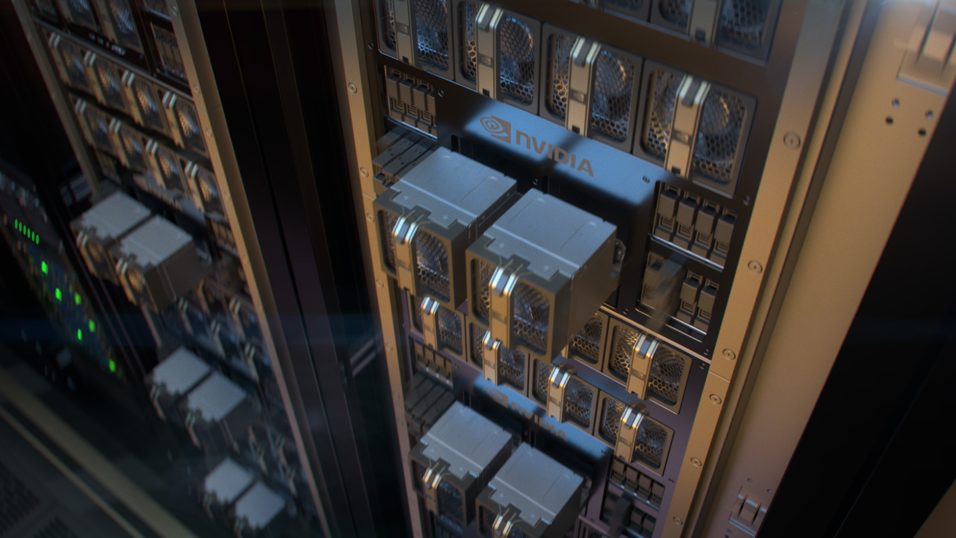
The GTC video performance showcases a digital twin NVIDIA is building of its own data centers — a virtual representation of the physical supercomputer that NVIDIA designers and engineers can use to test new configurations or software builds before releasing updates to the physical system.
In addition to enabling continuous integration and delivery, a digital twin of a data center can be used to optimize operational efficiency, including response time, resource utilization and energy consumption.
Digital twins can help teams predict equipment failures, proactively replace weak links and test improvement measures before applying them. They can even provide a testing ground to fine-tune data centers for specific enterprise users or applications.
Applicable across industries and applications, digital twin technology is already being used as a powerful tool for warehouse optimizations, climate simulations, smart factory development and renewable energy planning.
In NVIDIA’s data center digital twin, viewers can spot flagship technologies including NVIDIA DGX SuperPOD and EGX-based NVIDIA-Certified systems with BlueField DPUs and InfiniBand switches. The performance also features a special appearance by Toy Jensen, an application built with Omniverse Avatar.
The visualization was developed in NVIDIA Omniverse, a platform for real-time world simulation and 3D design collaboration. Omniverse connects science and art by bringing together creators, developers, engineers and AIs across industries to work together in a shared virtual world.
Omniverse digital twins are true to reality, accurately simulating the physics and materials of their real counterparts. The realism allows Omniverse users to test out processes, interactions and new technologies in the digital space before moving to the physical world.
Every factory, neighborhood and city could one day be replicated as a digital twin. With connected sensors powered by edge computing, these sandbox environments can be continuously updated to reflect changes to the corresponding real-world assets or systems. They can help develop next-generation autonomous robots, smart cities and 5G networks.
A digital twin can learn the laws of physics, chemistry, biology and more, storing this information in its computing brain.
Just as kingdoms centuries ago sent explorers to travel the world and return with new knowledge, edge sensors and robots are today’s explorers for digital twin environments. Each sensor brings new observations back to the digital twin’s brain, which consolidates the data, learns from it and updates the autonomous systems within the virtual environment. This collective learning will tune digital twins to perfection.
Hear about the latest innovations in AI, accelerated computing and virtual world simulation at GTC, streaming online through March 24. Register free and learn more about data center acceleration in the session replay, “How to Achieve Millionfold Speedups in Data Center Performance.” Watch NVIDIA founder and CEO Jensen Huang’s keynote address below:
The post Orchestrated to Perfection: NVIDIA Data Center Grooves to Tune of Millionfold Speedups appeared first on NVIDIA Blog.
Set up a text summarization project with Hugging Face Transformers: Part 2
This is the second post in a two-part series in which I propose a practical guide for organizations so you can assess the quality of text summarization models for your domain.
For an introduction to text summarization, an overview of this tutorial, and the steps to create a baseline for our project (also referred to as section 1), refer back to the first post.
This post is divided into three sections:
- Section 2: Generate summaries with a zero-shot model
- Section 3: Train a summarization model
- Section 4: Evaluate the trained model
Section 2: Generate summaries with a zero-shot model
In this post, we use the concept of zero-shot learning (ZSL), which means we use a model that has been trained to summarize text but hasn’t seen any examples of the arXiv dataset. It’s a bit like trying to paint a portrait when all you have been doing in your life is landscape painting. You know how to paint, but you might not be too familiar with the intricacies of portrait painting.
For this section, we use the following notebook.
Why zero-shot learning?
ZSL has become popular over the past years because it allows you to use state-of-the-art NLP models with no training. And their performance is sometimes quite astonishing: the Big Science Research Workgroup has recently released their T0pp (pronounced “T Zero Plus Plus”) model, which has been trained specifically for researching zero-shot multitask learning. It can often outperform models six times larger on the BIG-bench benchmark, and can outperform the GPT-3 (16 times larger) on several other NLP benchmarks.
Another benefit of ZSL is that it takes just two lines of code to use it. By trying it out, we create a second baseline, which we use to quantify the gain in model performance after we fine-tune the model on our dataset.
Set up a zero-shot learning pipeline
To use ZSL models, we can use Hugging Face’s Pipeline API. This API enables us to use a text summarization model with just two lines of code. It takes care of the main processing steps in an NLP model:
- Preprocess the text into a format the model can understand.
- Pass the preprocessed inputs to the model.
- Postprocess the predictions of the model, so you can make sense of them.
It uses the summarization models that are already available on the Hugging Face model hub.
To use it, run the following code:
That’s it! The code downloads a summarization model and creates summaries locally on your machine. If you’re wondering which model it uses, you can either look it up in the source code or use the following command:
When we run this command, we see that the default model for text summarization is called sshleifer/distilbart-cnn-12-6:

We can find the model card for this model on the Hugging Face website, where we can also see that the model has been trained on two datasets: the CNN Dailymail dataset and the Extreme Summarization (XSum) dataset. It’s worth noting that this model is not familiar with the arXiv dataset and is only used to summarize texts that are similar to the ones it has been trained on (mostly news articles). The numbers 12 and 6 in the model name refer to the number of encoder layers and decoder layers, respectively. Explaining what these are is outside the scope of this tutorial, but you can read more about it in the post Introducing BART by Sam Shleifer, who created the model.
We use the default model going forward, but I encourage you to try out different pre-trained models. All the models that are suitable for summarization can be found on the Hugging Face website. To use a different model, you can specify the model name when calling the Pipeline API:
Extractive vs. abstractive summarization
We haven’t spoken yet about two possible but different approaches to text summarization: extractive vs. abstractive. Extractive summarization is the strategy of concatenating extracts taken from a text into a summary, whereas abstractive summarization involves paraphrasing the corpus using novel sentences. Most of the summarization models are based on models that generate novel text (they’re natural language generation models, like, for example, GPT-3). This means that the summarization models also generate novel text, which makes them abstractive summarization models.
Generate zero-shot summaries
Now that we know how to use it, we want to use it on our test dataset—the same dataset we used in section 1 to create the baseline. We can do that with the following loop:
We use the min_length and max_length parameters to control the summary the model generates. In this example, we set min_length to 5 because we want the title to be at least five words long. And by estimating the reference summaries (the actual titles for the research papers), we determine that 20 could be a reasonable value for max_length. But again, this is just a first attempt. When the project is in the experimentation phase, these two parameters can and should be changed to see if the model performance changes.
Additional parameters
If you’re already familiar with text generation, you might know there are many more parameters to influence the text a model generates, such as beam search, sampling, and temperature. These parameters give you more control over the text that is being generated, for example make the text more fluent and less repetitive. These techniques are not available in the Pipeline API—you can see in the source code that min_length and max_length are the only parameters that are considered. After we train and deploy our own model, however, we have access to those parameters. More on that in section 4 of this post.
Model evaluation
After we have the generated the zero-shot summaries, we can use our ROUGE function again to compare the candidate summaries with the reference summaries:
Running this calculation on the summaries that were generated with the ZSL model gives us the following results:
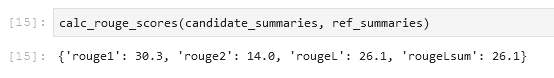
When we compare those with our baseline, we see that this ZSL model is actually performing worse that our simple heuristic of just taking the first sentence. Again, this is not unexpected: although this model knows how to summarize news articles, it has never seen an example of summarizing the abstract of an academic research paper.
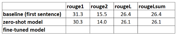
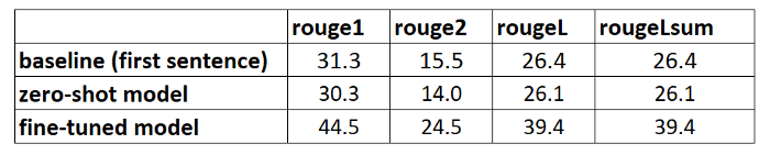
Baseline comparison
We have now created two baselines: one using a simple heuristic and one with an ZSL model. By comparing the ROUGE scores, we see that the simple heuristic currently outperforms the deep learning model.
In the next section, we take this same deep learning model and try to improve its performance. We do so by training it on the arXiv dataset (this step is also called fine-tuning). We take advantage of the fact that it already knows how to summarize text in general. We then show it lots of examples of our arXiv dataset. Deep learning models are exceptionally good at identifying patterns in datasets after they get trained on it, so we expect the model to get better at this particular task.
Section 3: Train a summarization model
In this section, we train the model we used for zero-shot summaries in section 2 (sshleifer/distilbart-cnn-12-6) on our dataset. The idea is to teach the model what summaries for abstracts of research papers look like by showing it many examples. Over time the model should recognize the patterns in this dataset, which will allow it to create better summaries.
It’s worth noting once more that if you have labeled data, namely texts and corresponding summaries, you should use those to train a model. Only by doing so can the model learn the patterns of your specific dataset.
The complete code for the model training is in the following notebook.
Set up a training job
Because training a deep learning model would take a few weeks on a laptop, we use Amazon SageMaker training jobs instead. For more details, refer to Train a Model with Amazon SageMaker. In this post, I briefly highlight the advantage of using these training jobs, besides the fact that they allow us to use GPU compute instances.
Let’s assume we have a cluster of GPU instances we can use. In that case, we likely want to create a Docker image to run the training so that we can easily replicate the training environment on other machines. We then install the required packages and because we want to use several instances, we need to set up distributed training as well. When the training is complete, we want to quickly shut down these computers because they are costly.
All these steps are abstracted away from us when using training jobs. In fact, we can train a model in the same way as described by specifying the training parameters and then just calling one method. SageMaker takes care of the rest, including stopping the GPU instances when the training is complete so to not incur any further costs.
In addition, Hugging Face and AWS announced a partnership earlier in 2022 that makes it even easier to train Hugging Face models on SageMaker. This functionality is available through the development of Hugging Face AWS Deep Learning Containers (DLCs). These containers include Hugging Face Transformers, Tokenizers and the Datasets library, which allows us to use these resources for training and inference jobs. For a list of the available DLC images, see available Hugging Face Deep Learning Containers Images. They are maintained and regularly updated with security patches. We can find many examples of how to train Hugging Face models with these DLCs and the Hugging Face Python SDK in the following GitHub repo.
We use one of those examples as a template because it does almost everything we need for our purpose: train a summarization model on a specific dataset in a distributed manner (using more than one GPU instance).
One thing, however, we have to account for is that this example uses a dataset directly from the Hugging Face dataset hub. Because we want to provide our own custom data, we need to amend the notebook slightly.
Pass data to the training job
To account for the fact that we bring our own dataset, we need to use channels. For more information, refer to How Amazon SageMaker Provides Training Information.
I personally find this term a bit confusing, so in my mind I always think mapping when I hear channels, because it helps me better visualize what happens. Let me explain: as we already learned, the training job spins up a cluster of Amazon Elastic Compute Cloud (Amazon EC2) instances and copies a Docker image onto it. However, our datasets are stored in Amazon Simple Storage Service (Amazon S3) and can’t be accessed by that Docker image. Instead, the training job needs to copy the data from Amazon S3 to a predefined path locally in that Docker image. The way it does that is by us telling the training job where the data resides in Amazon S3 and where on the Docker image the data should be copied to so that the training job can access it. We map the Amazon S3 location with the local path.
We set the local path in the hyperparameters section of the training job:
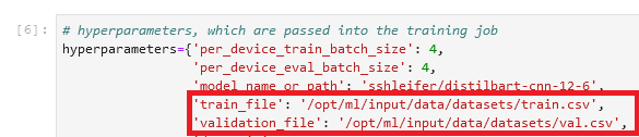
Then we tell the training job where the data resides in Amazon S3 when calling the fit() method, which starts the training:
![]()
Note that the folder name after /opt/ml/input/data matches the channel name (datasets). This enables the training job to copy the data from Amazon S3 to the local path.
Start the training
We’re now ready to start the training job. As mentioned before, we do so by calling the fit() method. The training job runs for about 40 minutes. You can follow the progress and see additional information on the SageMaker console.
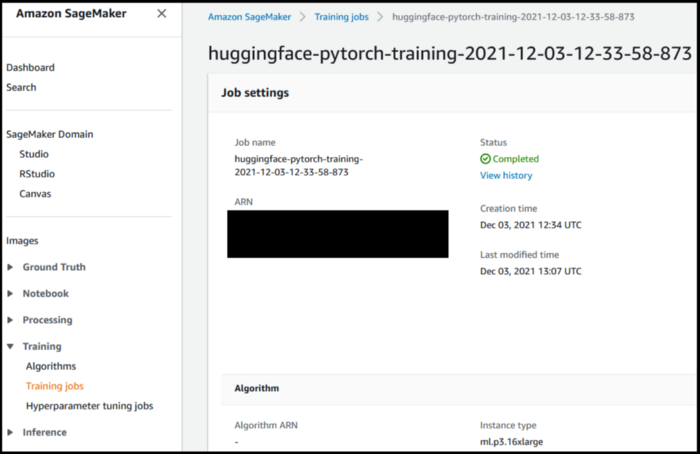
When the training job is complete, it’s time to evaluate our newly trained model.
Section 4: Evaluate the trained model
Evaluating our trained model is very similar to what we did in section 2, where we evaluated the ZSL model. We call the model and generate candidate summaries and compare them to the reference summaries by calculating the ROUGE scores. But now, the model sits in Amazon S3 in a file called model.tar.gz (to find the exact location, you can check the training job on the console). So how do we access the model to generate summaries?
We have two options: deploy the model to a SageMaker endpoint or download it locally, similar to what we did in section 2 with the ZSL model. In this tutorial, I deploy the model to a SageMaker endpoint because it’s more convenient and by choosing a more powerful instance for the endpoint, we can shorten the inference time significantly. The GitHub repo contains a notebook that shows how to evaluate the model locally.
Deploy a model
It’s usually very easy to deploy a trained model on SageMaker (see again the following example on GitHub from Hugging Face). After the model has been trained, we can call estimator.deploy() and SageMaker does the rest for us in the background. Because in our tutorial we switch from one notebook to the next, we have to locate the training job and the associated model first, before we can deploy it:

After we retrieve the model location, we can deploy it to a SageMaker endpoint:
Deployment on SageMaker is straightforward because it uses the SageMaker Hugging Face Inference Toolkit, an open-source library for serving Transformers models on SageMaker. We normally don’t even have to provide an inference script; the toolkit takes care of that. In that case, however, the toolkit utilizes the Pipeline API again, and as we discussed in section 2, the Pipeline API doesn’t allow us to use advanced text generation techniques such as beam search and sampling. To avoid this limitation, we provide our custom inference script.
First evaluation
For the first evaluation of our newly trained model, we use the same parameters as in section 2 with the zero-shot model to generate the candidate summaries. This allows to make an apple-to-apples comparison:
We compare the summaries generated by the model with the reference summaries:
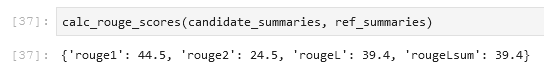
This is encouraging! Our first attempt to train the model, without any hyperparameter tuning, has improved the ROUGE scores significantly.
Second evaluation
Now it’s time to use some more advanced techniques such as beam search and sampling to play around with the model. For a detailed explanation what each of these parameters does, refer to How to generate text: using different decoding methods for language generation with Transformers. Let’s try it with a semi-random set of values for some of these parameters:
When running our model with these parameters, we get the following scores:

That didn’t work out quite as we hoped—the ROUGE scores have actually gone down slightly. However, don’t let this discourage you from trying out different values for these parameters. In fact, this is the point where we finish with the setup phase and transition into the experimentation phase of the project.
Conclusion and next steps
We have concluded the setup for the experimentation phase. In this two-part series, we downloaded and prepared our data, created a baseline with a simple heuristic, created another baseline using zero-shot learning, and then trained our model and saw a significant increase in performance. Now it’s time to play around with every part we created in order to create even better summaries. Consider the following:
- Preprocess the data properly – For example, remove stopwords and punctuation. Don’t underestimate this part—in many data science projects, data preprocessing is one of the most important aspects (if not the most important), and data scientists typically spend most of their time with this task.
-
Try out different models – In our tutorial, we used the standard model for summarization (
sshleifer/distilbart-cnn-12-6), but many more models are available that you can use for this task. One of those might better fit your use case. - Perform hyperparameter tuning – When training the model, we used a certain set of hyperparameters (learning rate, number of epochs, and so on). These parameters aren’t set in stone—quite the opposite. You should change these parameters to understand how they affect your model performance.
- Use different parameters for text generation – We already did one round of creating summaries with different parameters to utilize beam search and sampling. Try out different values and parameters. For more information, refer to How to generate text: using different decoding methods for language generation with Transformers.
I hope you made it to the end and found this tutorial useful.
About the Author
 Heiko Hotz is a Senior Solutions Architect for AI & Machine Learning and leads the Natural Language Processing (NLP) community within AWS. Prior to this role, he was the Head of Data Science for Amazon’s EU Customer Service. Heiko helps our customers being successful in their AI/ML journey on AWS and has worked with organizations in many industries, including Insurance, Financial Services, Media and Entertainment, Healthcare, Utilities, and Manufacturing. In his spare time Heiko travels as much as possible.
Set up a text summarization project with Hugging Face Transformers: Part 1
When OpenAI released the third generation of their machine learning (ML) model that specializes in text generation in July 2020, I knew something was different. This model struck a nerve like no one that came before it. Suddenly I heard friends and colleagues, who might be interested in technology but usually don’t care much about the latest advancements in the AI/ML space, talk about it. Even the Guardian wrote an article about it. Or, to be precise, the model wrote the article and the Guardian edited and published it. There was no denying it – GPT-3 was a game changer.
After the model had been released, people immediately started to come up with potential applications for it. Within weeks, many impressive demos were created, which can be found on the GPT-3 website. One particular application that caught my eye was text summarization – the capability of a computer to read a given text and summarize its content. It’s one of the hardest tasks for a computer because it combines two fields within the field of natural language processing (NLP): reading comprehension and text generation. Which is why I was so impressed by the GPT-3 demos for text summarization.
You can give them a try on the Hugging Face Spaces website. My favorite one at the moment is an application that generates summaries of news articles with just the URL of the article as input.
In this two-part series, I propose a practical guide for organizations so you can assess the quality of text summarization models for your domain.
Tutorial overview
Many organizations I work with (charities, companies, NGOs) have huge amounts of texts they need to read and summarize – financial reports or news articles, scientific research papers, patent applications, legal contracts, and more. Naturally, these organizations are interested in automating these tasks with NLP technology. To demonstrate the art of the possible, I often use the text summarization demos, which almost never fail to impress.
But now what?
The challenge for these organizations is that they want to assess text summarization models based on summaries for many, many documents – not one at a time. They don’t want to hire an intern whose only job is to open the application, paste in a document, hit the Summarize button, wait for the output, assess whether the summary is good, and do that all over again for thousands of documents.
I wrote this tutorial with my past self from four weeks ago in mind – it’s the tutorial I wish I had back then when I started on this journey. In that sense, the target audience of this tutorial is someone who is familiar with AI/ML and has used Transformer models before, but is at the beginning of their text summarization journey and wants to dive deeper into it. Because it’s written by a “beginner” and for beginners, I want to stress the fact that this tutorial is a practical guide – not the practical guide. Please treat it as if George E.P. Box had said:
In terms of how much technical knowledge is required in this tutorial: It does involve some coding in Python, but most of the time we just use the code to call APIs, so no deep coding knowledge is required, either. It’s helpful to be familiar with certain concepts of ML, such as what it means to train and deploy a model, the concepts of training, validation, and test datasets, and so on. Also having dabbled with the Transformers library before might be useful, because we use this library extensively throughout this tutorial. I also include useful links for further reading for these concepts.
Because this tutorial is written by a beginner, I don’t expect NLP experts and advanced deep learning practitioners to get much of this tutorial. At least not from a technical perspective – you might still enjoy the read, though, so please don’t leave just yet! But you will have to be patient with regards to my simplifications – I tried to live by the concept of making everything in this tutorial as simple as possible, but not simpler.
Structure of this tutorial
This series stretches over four sections split into two posts, in which we go through different stages of a text summarization project. In the first post (section 1), we start by introducing a metric for text summarization tasks – a measure of performance that allows us to assess whether a summary is good or bad. We also introduce the dataset we want to summarize and create a baseline using a no-ML model – we use a simple heuristic to generate a summary from a given text. Creating this baseline is a vitally important step in any ML project because it enables us to quantify how much progress we make by using AI going forward. It allows us to answer the question “Is it really worth investing in AI technology?”
In the second post, we use a model that already has been pre-trained to generate summaries (section 2). This is possible with a modern approach in ML called transfer learning. It’s another useful step because we basically take an off-the-shelf model and test it on our dataset. This allows us to create another baseline, which helps us see what happens when we actually train the model on our dataset. The approach is called zero-shot summarization, because the model has had zero exposure to our dataset.
After that, it’s time to use a pre-trained model and train it on our own dataset (section 3). This is also called fine-tuning. It enables the model to learn from the patterns and idiosyncrasies of our data and slowly adapt to it. After we train the model, we use it to create summaries (section 4).
To summarize:
- Part 1:
- Section 1: Use a no-ML model to establish a baseline
-
Part 2:
- Section 2: Generate summaries with a zero-shot model
- Section 3: Train a summarization model
- Section 4: Evaluate the trained model
The entire code for this tutorial is available in the following GitHub repo.
What will we have achieved by the end of this tutorial?
By the end of this tutorial, we won’t have a text summarization model that can be used in production. We won’t even have a good summarization model (insert scream emoji here)!
What we will have instead is a starting point for the next phase of the project, which is the experimentation phase. This is where the “science” in data science comes in, because now it’s all about experimenting with different models and different settings to understand whether a good enough summarization model can be trained with the available training data.
And, to be completely transparent, there is a good chance that the conclusion will be that the technology is just not ripe yet and that the project will not be implemented. And you have to prepare your business stakeholders for that possibility. But that’s a topic for another post.
Section 1: Use a no-ML model to establish a baseline
This is the first section of our tutorial on setting up a text summarization project. In this section, we establish a baseline using a very simple model, without actually using ML. This is a very important step in any ML project, because it allows us to understand how much value ML adds over the time of the project and if it’s worth investing in it.
The code for the tutorial can be found in the following GitHub repo.
Data, data, data
Every ML project starts with data! If possible, we always should use data related to what we want to achieve with a text summarization project. For example, if our goal is to summarize patent applications, we should also use patent applications to train the model. A big caveat for an ML project is that the training data usually needs to be labeled. In the context of text summarization, that means we need to provide the text to be summarized as well as the summary (the label). Only by providing both can the model learn what a good summary looks like.
In this tutorial, we use a publicly available dataset, but the steps and code remain exactly the same if we use a custom or private dataset. And again, if you have an objective in mind for your text summarization model and have corresponding data, please use your data instead to get the most out of this.
The data we use is the arXiv dataset, which contains abstracts of arXiv papers as well as their titles. For our purpose, we use the abstract as the text we want to summarize and the title as the reference summary. All the steps of downloading and preprocessing the data are available in the following notebook. We require an AWS Identity and Access Management (IAM) role that permits loading data to and from Amazon Simple Storage Service (Amazon S3) in order to run this notebook successfully. The dataset was developed as part of the paper On the Use of ArXiv as a Dataset and is licensed under the Creative Commons CC0 1.0 Universal Public Domain Dedication.
The data is split into three datasets: training, validation, and test data. If you want to use your own data, make sure this is the case too. The following diagram illustrates how we use the different datasets.
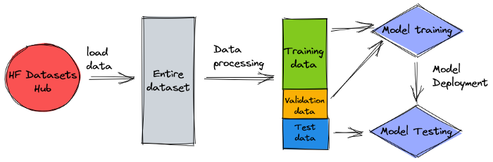
Naturally, a common question at this point is: How much data do we need? As you can probably already guess, the answer is: it depends. It depends on how specialized the domain is (summarizing patent applications is quite different from summarizing news articles), how accurate the model needs to be to be useful, how much the training of the model should cost, and so on. We return to this question at a later point when we actually train the model, but the short of it is that we have to try out different dataset sizes when we’re in the experimentation phase of the project.
What makes a good model?
In many ML projects, it’s rather straightforward to measure a model’s performance. That’s because there is usually little ambiguity around whether the model’s result is correct. The labels in the dataset are often binary (True/False, Yes/No) or categorical. In any case, it’s easy in this scenario to compare the model’s output to the label and mark it as correct or incorrect.
When generating text, this becomes more challenging. The summaries (the labels) we provide in our dataset are only one way to summarize text. But there are many possibilities to summarize a given text. So, even if the model doesn’t match our label 1:1, the output might still be a valid and useful summary. So how do we compare the model’s summary with the one we provide? The metric that is used most often in text summarization to measure the quality of a model is the ROUGE score. To understand the mechanics of this metric, refer to The Ultimate Performance Metric in NLP. In summary, the ROUGE score measures the overlap of n-grams (contiguous sequence of n items) between the model’s summary (candidate summary) and the reference summary (the label we provide in our dataset). But, of course, this is not a perfect measure. To understand its limitations, check out To ROUGE or not to ROUGE?
So, how do we calculate the ROUGE score? There are quite a few Python packages out there to compute this metric. To ensure consistency, we should use the same method throughout our project. Because we will, at a later point in this tutorial, use a training script from the Transformers library instead of writing our own, we can just peek into the source code of the script and copy the code that computes the ROUGE score:
By using this method to compute the score, we ensure that we always compare apples to apples throughout the project.
This function computes several ROUGE scores: rouge1, rouge2, rougeL, and rougeLsum. The “sum” in rougeLsum refers to the fact that this metric is computed over a whole summary, whereas rougeL is computed as the average over individual sentences. So, which ROUGE score we should use for our project? Again, we have to try different approaches in the experimentation phase. For what it’s worth, the original ROUGE paper states that “ROUGE-2 and ROUGE-L worked well in single document summarization tasks” while “ROUGE-1 and ROUGE-L perform great in evaluating short summaries.”
Create the baseline
Next up we want to create the baseline by using a simple, no-ML model. What does that mean? In the field of text summarization, many studies use a very simple approach: they take the first n sentences of the text and declare it the candidate summary. They then compare the candidate summary with the reference summary and compute the ROUGE score. This is a simple yet powerful approach that we can implement in a few lines of code (the entire code for this part is in the following notebook):
We use the test dataset for this evaluation. This makes sense because after we train the model, we also use the same test dataset for the final evaluation. We also try different numbers for n: we start with only the first sentence as the candidate summary, then the first two sentences, and finally the first three sentences.
The following screenshot shows the results for our first model.
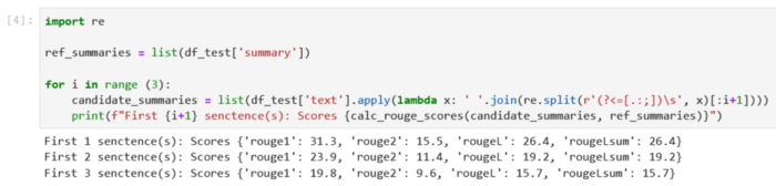
The ROUGE scores are highest, with only the first sentence as the candidate summary. This means that taking more than one sentence makes the summary too verbose and leads to a lower score. So that means we will use the scores for the one-sentence summaries as our baseline.
It’s important to note that, for such a simple approach, these numbers are actually quite good, especially for the rouge1 score. To put these numbers in context, we can refer to Pegasus Models, which shows the scores of a state-of-the-art model for different datasets.
Conclusion and what’s next
In Part 1 of our series, we introduced the dataset that we use throughout the summarization project as well as a metric to evaluate summaries. We then created the following baseline with a simple, no-ML model.
In the next post, we use a zero-shot model – specifically, a model that has been specifically trained for text summarization on public news articles. However, this model won’t be trained at all on our dataset (hence the name “zero-shot”).
I leave it to you as homework to guess on how this zero-shot model will perform compared to our very simple baseline. On the one hand, it will be a much more sophisticated model (it’s actually a neural network). On the other hand, it’s only used to summarize news articles, so it might struggle with the patterns that are inherent to the arXiv dataset.
About the Author
Heiko Hotz is a Senior Solutions Architect for AI & Machine Learning and leads the Natural Language Processing (NLP) community within AWS. Prior to this role, he was the Head of Data Science for Amazon’s EU Customer Service. Heiko helps our customers being successful in their AI/ML journey on AWS and has worked with organizations in many industries, including Insurance, Financial Services, Media and Entertainment, Healthcare, Utilities, and Manufacturing. In his spare time Heiko travels as much as possible.
Optimize customer engagement with reinforcement learning
This is a guest post co-authored by Taylor Names, Staff Machine Learning Engineer, Dev Gupta, Machine Learning Manager, and Argie Angeleas, Senior Product Manager at Ibotta. Ibotta is an American technology company that enables users with its desktop and mobile apps to earn cash back on in-store, mobile app, and online purchases with receipt submission, linked retailer loyalty accounts, payments, and purchase verification.
Ibotta strives to recommend personalized promotions to better retain and engage its users. However, promotions and user preferences are constantly evolving. This ever-changing environment with many new users and new promotions is a typical cold start problem—there is no sufficient historical user and promotion interactions to draw any inferences from. Reinforcement learning (RL) is an area of machine learning (ML) concerned with how intelligent agents should take action in an environment in order to maximize the notion of cumulative rewards. RL focuses on finding a balance between exploring uncharted territory and exploiting current knowledge. Multi-armed bandit (MAB) is a classic reinforcement learning problem that exemplifies the exploration/exploitation tradeoff: maximizing reward in the short-term (exploitation) while sacrificing the short-term reward for knowledge that can increase rewards in the long term (exploration). A MAB algorithm explores and exploits optimal recommendations for the user.
Ibotta collaborated with the Amazon Machine Learning Solutions Lab to use MAB algorithms to increase user engagement when the user and promotion information is highly dynamic.
We selected a contextual MAB algorithm because it’s effective in the following use cases:
- Making personalized recommendations according to users’ state (context)
- Dealing with cold start aspects such as new bonuses and new customers
- Accommodating recommendations where users’ preferences change over time
Data
To increase bonus redemptions, Ibotta desires to send personalized bonuses to customers. Bonuses are Ibotta’s self-funded cash incentives, which serve as the actions of the contextual multi-armed bandit model.
The bandit model uses two sets of features:
- Action features – These describe the actions, such as bonus type and average amount of the bonus
- Customer features – These describe customers’ historical preferences and interactions, such as past weeks’ redemptions, clicks, and views
The contextual features are derived from historical customer journeys, which contained 26 weekly activity metrics generated from users’ interactions with the Ibotta app.
Contextual multi-armed bandit
Bandit is a framework for sequential decision-making in which the decision-maker sequentially chooses an action, potentially based on the current contextual information, and observes a reward signal.
We set up the contextual multi-armed bandit workflow on Amazon SageMaker using the built-in Vowpal Wabbit (VW) container. SageMaker helps data scientists and developers prepare, build, train, and deploy high-quality ML models quickly by bringing together a broad set of capabilities purpose-built for ML. The model training and testing are based on offline experimentation. The bandit learns user preferences based on their feedback from past interactions rather than a live environment. The algorithm can switch to production mode, where SageMaker remains as the supporting infrastructure.
To implement the exploration/exploitation strategy, we built the iterative training and deployment system that performs the following actions:
- Recommends an action using the contextual bandit model based on user context
- Captures the implicit feedback over time
- Continuously trains the model with incremental interaction data
The workflow of the client application is as follows:
- The client application picks a context, which is sent to the SageMaker endpoint to retrieve an action.
- The SageMaker endpoint returns an action, associated bonus redemption probability, and
event_id. - Because this simulator was generated using historical interactions, the model knows the true class for that context. If the agent selects an action with redemption, the reward is 1. Otherwise, the agent obtains a reward of 0.
In the case where historical data is available and is in the format of <state, action, action probability, reward>, Ibotta can warm start a live model by learning the policy offline. Otherwise, Ibotta can initiate a random policy for day 1 and start to learn a bandit policy from there.
The following is the code snippet to train the model:
Model performance
We randomly split the redeemed interactions as training data (10,000 interactions) and evaluation data (5,300 holdout interactions).
Evaluation metrics are the mean reward, where 1 indicates the recommended action was redeemed, and 0 indicates the recommended action didn’t get redeemed.
We can determine the mean reward as follows:
Mean reward (redeem rate) = (# of recomended actions with redemption)/(total # recommended actions)
The following table shows the mean reward result:
| Mean Reward | Uniform Random Recommendation | Contextual MAB-based Recommendation |
| Train | 11.44% | 56.44% |
| Test | 10.69% | 59.09% |
The following figure plots the incremental performance evaluation during training, where the x-axis is the number of records learned by the model and the y-axis is the incremental mean reward. The blue line indicates the multi-armed bandit; the orange line indicates random recommendations.
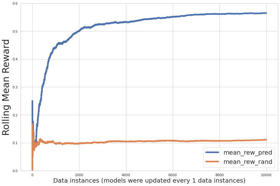
The graph shows that the predicted mean reward increases over the iterations, and the predicted action reward is significantly greater than the random assignment of actions.
We can use previously trained models as warm starts and batch retrain the model with new data. In this case, model performance already converged through initial training. No significant additional performance improvement was observed in new batch retraining, as shown in the following figure.

We also compared contextual bandit with uniformly random and posterior random (random recommendation using historical user preference distribution as warm start) policies. The results are listed and plotted as follows:
- Bandit – 59.09% mean reward (training 56.44%)
- Uniform random – 10.69% mean reward (training 11.44%)
- Posterior probability random – 34.21% mean reward (training 34.82%)
The contextual multi-armed bandit algorithm outperformed the other two policies significantly.

Summary
The Amazon ML Solutions Lab collaborated with Ibotta to develop a contextual bandit reinforcement learning recommendation solution using a SageMaker RL container.
This solution demonstrated a steady incremental redemption rate lift over random (five-times lift) and non-contextual RL (two-times lift) recommendations based on an offline test. With this solution, Ibotta can establish a dynamic user-centric recommendation engine to optimize customer engagement. Compared to random recommendation, the solution improved recommendation accuracy (mean reward) from 11% to 59%, according to the offline test. Ibotta plans to integrate this solution into more personalization use cases.
“The Amazon ML Solutions Lab worked closely with Ibotta’s Machine Learning team to build a dynamic bonus recommendation engine to increase redemptions and optimize customer engagement. We created a recommendation engine leveraging reinforcement learning that learns and adapts to the ever-changing customer state and cold starts new bonuses automatically. Within 2 months, the ML Solutions Lab scientists developed a contextual multi-armed bandit reinforcement learning solution using a SageMaker RL container. The contextual RL solution showed a steady increase in redemption rates, achieving a five-times lift in bonus redemption rate over random recommendation, and a two-times lift over a non-contextual RL solution. The recommendation accuracy improved from 11% using random recommendation to 59% using the ML Solutions Lab solution. Given the effectiveness and flexibility of this solution, we plan to integrate this solution into more Ibotta personalization use cases to further our mission of making every purchase rewarding for our users.”
– Heather Shannon, Senior Vice President of Engineering & Data at Ibotta.
About the Authors
 Taylor Names is a staff machine learning engineer at Ibotta, focusing on content personalization and real-time demand forecasting. Prior to joining Ibotta, Taylor led machine learning teams in the IoT and clean energy spaces.
 Dev Gupta is an engineering manager at Ibotta Inc, where he leads the machine learning team. The ML team at Ibotta is tasked with providing high-quality ML software, such as recommenders, forecasters, and internal ML tools. Before joining Ibotta, Dev worked at Predikto Inc, a machine learning startup, and The Home Depot. He graduated from the University of Florida.
 Argie Angeleas is a Senior Product Manager at Ibotta, where he leads the Machine Learning and Browser Extension squads. Before joining Ibotta, Argie worked as Director of Product at iReportsource. Argie obtained his PhD in Computer Science and Engineering from Wright State University.
 Fang Wang is a Senior Research Scientist at the Amazon Machine Learning Solutions Lab, where she leads the Retail Vertical, working with AWS customers across various industries to solve their ML problems. Before joining AWS, Fang worked as Sr. Director of Data Science at Anthem, leading the medical claim processing AI platform. She obtained her master’s in Statistics from the University of Chicago.
 Xin Chen is a senior manager at the Amazon Machine Learning Solutions Lab, where he leads the Central US, Greater China Region, LATAM, and Automotive Vertical. He helps AWS customers across different industries identify and build machine learning solutions to address their organization’s highest return-on-investment machine learning opportunities. Xin obtained his PhD in Computer Science and Engineering from the University of Notre Dame.
 Raj Biswas is a Data Scientist at the Amazon Machine Learning Solutions Lab. He helps AWS customers develop ML-powered solutions across diverse industry verticals for their most pressing business challenges. Prior to joining AWS, he was a graduate student at Columbia University in Data Science.
 Xinghua Liang is an Applied Scientist at the Amazon Machine Learning Solutions Lab, where he works with customers across various industries, including manufacturing and automotive, and helps them to accelerate their AI and cloud adoption. Xinghua obtained his PhD in Engineering from Carnegie Mellon University.
 Yi Liu is an applied scientist with Amazon Customer Service. She is passionate about using the power of ML/AI to optimize user experience for Amazon customers and help AWS customers build scalable cloud solutions. Her science work in Amazon spans membership engagement, online recommendation system, and customer experience defect identification and resolution. Outside of work, Yi enjoys traveling and exploring nature with her dog.
Auto-generated Summaries in Google Docs
For many of us, it can be challenging to keep up with the volume of documents that arrive in our inboxes every day: reports, reviews, briefs, policies and the list goes on. When a new document is received, readers often wish it included a brief summary of the main points in order to effectively prioritize it. However, composing a document summary can be cognitively challenging and time-consuming, especially when a document writer is starting from scratch.
To help with this, we recently announced that Google Docs now automatically generates suggestions to aid document writers in creating content summaries, when they are available. Today we describe how this was enabled using a machine learning (ML) model that comprehends document text and, when confident, generates a 1-2 sentence natural language description of the document content. However, the document writer maintains full control — accepting the suggestion as-is, making necessary edits to better capture the document summary or ignoring the suggestion altogether. Readers can also use this section, along with the outline, to understand and navigate the document at a high level. While all users can add summaries, auto-generated suggestions are currently only available to Google Workspace business customers. Building on grammar suggestions, Smart Compose, and autocorrect, we see this as another valuable step toward improving written communication in the workplace.
 |
| A blue summary icon appears in the top left corner when a document summary suggestion is available. Document writers can then view, edit, or ignore the suggested document summary. |
Model Details
Automatically generated summaries would not be possible without the tremendous advances in ML for natural language understanding (NLU) and natural language generation (NLG) over the past five years, especially with the introduction of Transformer and Pegasus.
Abstractive text summarization, which combines the individually challenging tasks of long document language understanding and generation, has been a long-standing problem in NLU and NLG research. A popular method for combining NLU and NLG is training an ML model using sequence-to-sequence learning, where the inputs are the document words, and the outputs are the summary words. A neural network then learns to map input tokens to output tokens. Early applications of the sequence-to-sequence paradigm used recurrent neural networks (RNNs) for both the encoder and decoder.
The introduction of Transformers provided a promising alternative to RNNs because Transformers use self-attention to provide better modeling of long input and output dependencies, which is critical in document summarization. Still, these models require large amounts of manually labeled data to train sufficiently, so the advent of Transformers alone was not enough to significantly advance the state-of-the-art in document summarization.
The combination of Transformers with self-supervised pre-training (e.g., BERT, GPT, T5) led to a major breakthrough in many NLU tasks for which limited labeled data is available. In self-supervised pre-training, a model uses large amounts of unlabeled text to learn general language understanding and generation capabilities. Then, in a subsequent fine-tuning stage, the model learns to apply these abilities on a specific task, such as summarization or question answering.
The Pegasus work took this idea one step further, by introducing a pre-training objective customized to abstractive summarization. In Pegasus pre-training, also called Gap Sentence Prediction (GSP), full sentences from unlabeled news articles and web documents are masked from the input and the model is required to reconstruct them, conditioned on the remaining unmasked sentences. In particular, GSP attempts to mask sentences that are considered essential to the document through different heuristics. The intuition is to make the pre-training as close as possible to the summarization task. Pegasus achieved state-of-the-art results on a varied set of summarization datasets. However, a number of challenges remained to apply this research advancement into a product.
Applying Recent Research Advances to Google Docs
-
Data
Self-supervised pre-training results in an ML model that has general language understanding and generation capabilities, but a subsequent fine-tuning stage is critical for the model to adapt to the application domain. We fine-tuned early versions of our model on a corpus of documents with manually-generated summaries that were consistent with typical use cases.
However, early versions of this corpus suffered from inconsistencies and high variation because they included many types of documents, as well as many ways to write a summary — e.g., academic abstracts are typically long and detailed, while executive summaries are brief and punchy. This led to a model that was easily confused because it had been trained on so many different types of documents and summaries that it struggled to learn the relationships between any of them.
Fortunately, one of the key findings in the Pegasus work was that an effective pre-training phase required less supervised data in the fine-tuning stage. Some summarization benchmarks required as few as 1,000 fine-tuning examples for Pegasus to match the performance of Transformer baselines that saw 10,000+ supervised examples — suggesting that one could focus on quality rather than quantity.
We carefully cleaned and filtered the fine-tuning data to contain training examples that were more consistent and represented a coherent definition of summaries. Despite the fact that we reduced the amount of training data, this led to a higher quality model. The key lesson, consistent with recent work in domains like dataset distillation, was that it was better to have a smaller, high quality dataset, than a larger, high-variance dataset.


-
Serving
Once we trained the high quality model, we turned to the challenge of serving the model in production. While the Transformer version of the encoder-decoder architecture is the dominant approach to train models for sequence-to-sequence tasks like abstractive summarization, it can be inefficient and impractical to serve in real-world applications. The main inefficiency comes from the Transformer decoder where we generate the output summary token by token through autoregressive decoding. The decoding process becomes noticeably slow when summaries get longer since the decoder attends to all previously generated tokens at each step. RNNs are a more efficient architecture for decoding since there is no self-attention with previous tokens as in a Transformer model.
We used knowledge distillation, which is the process of transferring knowledge from a large model to a smaller more efficient model, to distill the Pegasus model into a hybrid architecture of a Transformer encoder and an RNN decoder. To improve efficiency we also reduced the number of RNN decoder layers. The resulting model had significant improvements in latency and memory footprint while the quality was still on par with the original model. To further improve the latency and user experience, we serve the summarization model using TPUs, which provide significant speed ups and allow more requests to be handled by a single machine.
Ongoing Challenges and Next Steps
While we are excited by the progress so far, there are a few challenges we are continuing to tackle:
- Document coverage: Developing a set of documents for the fine-tuning stage was difficult due to the tremendous variety that exists among documents, and the same challenge is true at inference time. Some of the documents our users create (e.g., meeting notes, recipes, lesson plans and resumes) are not suitable for summarization or can be difficult to summarize. Currently, our model only suggests a summary for documents where it is most confident, but we hope to continue broadening this set as our model improves.
- Evaluation: Abstractive summaries need to capture the essence of a document while being fluent and grammatically correct. A specific document may have many summaries that can be considered correct, and different readers may prefer different ones. This makes it hard to evaluate summaries with automatic metrics only, user feedback and usage statistics will be critical for us to understand and keep improving quality.
- Long documents: Long documents are some of the toughest documents for the model to summarize because it is harder to capture all the points and abstract them in a single summary, and it can also significantly increase memory usage during training and serving. However, long documents are perhaps most useful for the model to automatically summarize because it can help document writers get a head start on this tedious task. We hope we can apply the latest ML advancements to better address this challenge.
Conclusion
Overall, we are thrilled that we can apply recent progress in NLU and NLG to continue assisting users with reading and writing. We hope the automatic suggestions now offered in Google Workspace make it easier for writers to annotate their documents with summaries, and help readers comprehend and navigate documents more easily.
Acknowledgements
The authors would like to thank the many people across Google that contributed to this work: AJ Motika, Matt Pearson-Beck, Mia Chen, Mahdis Mahdieh, Halit Erdogan, Benjamin Lee, Ali Abdelhadi, Michelle Danoff, Vishnu Sivaji, Sneha Keshav, Aliya Baptista, Karishma Damani, DJ Lick, Yao Zhao, Peter Liu, Aurko Roy, Yonghui Wu, Shubhi Sareen, Andrew Dai, Mekhola Mukherjee, Yinan Wang, Mike Colagrosso, and Behnoosh Hariri. .

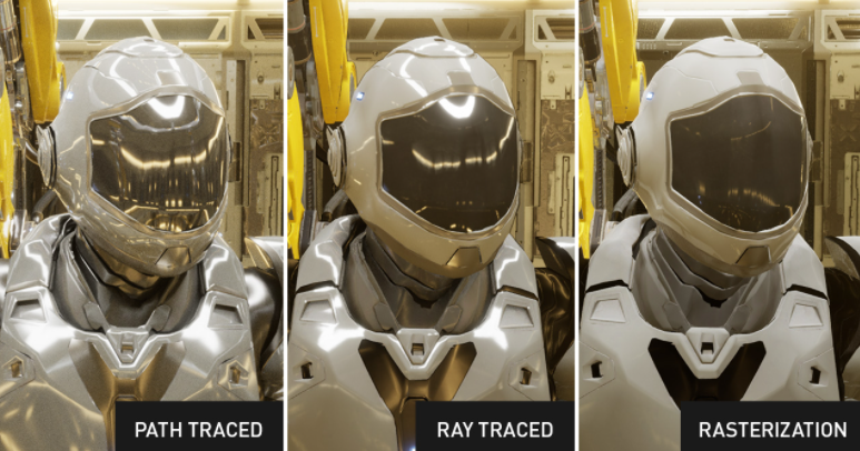
What Is Path Tracing?
Turn on your TV. Fire up your favorite streaming service. Grab a Coke. A demo of the most important visual technology of our time is as close as your living room couch.
Propelled by an explosion in computing power over the past decade and a half, path tracing has swept through visual media.
It brings big effects to the biggest blockbusters, casts subtle light and shadow on the most immersive melodramas and has propelled the art of animation to new levels.
More’s coming.
Path tracing is going real time, unleashing interactive, photorealistic 3D environments filled with dynamic light and shadow, reflections and refractions.
So what is path tracing? The big idea behind it is seductively simple, connecting innovators in the arts and sciences over the span half a millennium.
What’s the Difference Between Rasterization and Ray Tracing?
First, let’s define some terms, and how they’re used today to create interactive graphics — graphics that can react in real time to input from a user, such as in video games.
The first, rasterization, is a technique that produces an image as seen from a single viewpoint. It’s been at the heart of GPUs from the start. Modern NVIDIA GPUs can generate over 100 billion rasterized pixels per second. That’s made rasterization ideal for real-time graphics, like gaming.
Ray tracing is a more powerful technique than rasterization. Rather than being constrained to finding out what is visible from a single point, it can determine what is visible from many different points, in many different directions. Starting with the NVIDIA Turing architecture, NVIDIA GPUs have provided specialized RTX hardware to accelerate this difficult computation. Today, a single GPU can trace billions of rays per second.
Being able to trace all of those rays makes it possible to simulate how light scatters in the real world much more accurately than is possible with rasterization. However, we still must answer the questions, how will we simulate light and how will we bring that simulation to the GPU?
What’s Ray Tracing? Just Follow the String
To better answer that question, it helps to understand how we got here.
David Luebke, NVIDIA vice president of graphics research, likes to begin the story in the 16th century with Albrecht Dürer — one of the most important figures of the Northern European Renaissance — who used string and weights to replicate a 3D image on a 2D surface.
Dürer made it his life’s work to bring classical and contemporary mathematics together with the arts, achieving breakthroughs in expressiveness and realism.
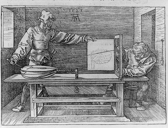
In 1538 with Treatise on Measurement, Dürer was the first to describe the idea of ray tracing. Seeing how Dürer described the idea is the easiest way to get your head around the concept.
Just think about how light illuminates the world we see around us.
Now imagine tracing those rays of light backward from the eye with a piece of string like the one Dürer used, to the objects that light interacts with. That’s ray tracing.
Ray Tracing for Computer Graphics
In 1969, more than 400 years after Dürer’s death, IBM’s Arthur Appel showed how the idea of ray tracing could be brought to computer graphics, applying it to computing visibility and shadows.
A decade later, Turner Whitted was the first to show how this idea could capture reflection, shadows and refraction, explaining how the seemingly simple concept could make much more sophisticated computer graphics possible. Progress was rapid in the following few years.
In 1984, Lucasfilm’s Robert Cook, Thomas Porter and Loren Carpenter detailed how ray tracing could incorporate many common filmmaking techniques — including motion blur, depth of field, penumbras, translucency and fuzzy reflections — that were, until then, unattainable in computer graphics.
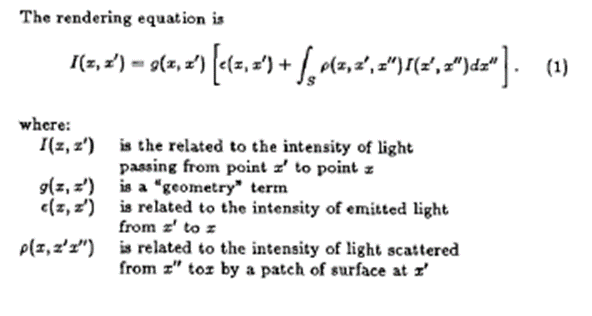
Two years later, CalTech professor Jim Kajiya’s crisp, seven-page paper, “The Rendering Equation,” connected computer graphics with physics by way of ray tracing and introduced the path-tracing algorithm, which makes it possible to accurately represent the way light scatters throughout a scene.
What’s Path Tracing?
In developing path tracing, Kajiya turned to an unlikely inspiration: the study of radiative heat transfer, or how heat spreads throughout an environment. Ideas from that field led him to introduce the rendering equation, which describes how light passes through the air and scatters from surfaces.
The rendering equation is concise, but not easy to solve. Computer graphics scenes are complex, with billions of triangles not being unusual today. There’s no way to solve the rendering equation directly, which led to Kajiya’s second crucial innovation.
Kajiya showed that statistical techniques could be used to solve the rendering equation: even if it isn’t solved directly, it’s possible to solve it along the paths of individual rays. If it is solved along the path of enough rays to approximate the lighting in the scene accurately, photorealistic images are possible.
And how is the rendering equation solved along the path of a ray? Ray tracing.
The statistical techniques Kajiya applied are known as Monte Carlo integration and date to the earliest days of computers in the 1940s. Developing improved Monte Carlo algorithms for path tracing remains an open research problem to this day; NVIDIA researchers are at the forefront of this area, regularly publishing new techniques that improve the efficiency of path tracing.
By putting these two ideas together — a physics-based equation for describing the way light moves around a scene — and the use of Monte Carlo simulation to help choose a manageable number of paths back to a light source, Kajiya outlined the fundamental techniques that would become the standard for generating photorealistic computer-generated images.
His approach transformed a field dominated by a variety of disparate rendering techniques into one that — because it mirrored the physics of the way light moved through the real world — could put simple, powerful algorithms to work that could be applied to reproduce a large number of visual effects with stunning levels of realism.
Path Tracing Comes to the Movies
In the years after its introduction in 1987, path tracing was seen as an elegant technique — the most accurate approach known — but it was completely impractical. The images in Kajiya’s original paper were just 256 by 256 pixels, yet they took over 7 hours to render on an expensive mini-computer that was far more powerful than the computers available to most other people.
But with the increase in computing power driven by Moore’s law — which described the exponential increase in computing power driven by advances that allowed chipmakers to double the number of transistors on microprocessors every 18 months — the technique became more and more practical.
Beginning with movies such as 1998’s A Bug’s Life, ray tracing was used to enhance the computer-generated imagery in more and more motion pictures. And in 2006, the first entirely path-traced movie, Monster House, stunned audiences. It was rendered using the Arnold software that was co-developed at Solid Angle SL (since acquired by Autodesk) and Sony Pictures Imageworks.
The film was a hit — grossing more than $140 million worldwide. And it opened eyes about what a new generation of computer animation could do. As more computing power became available, more movies came to rely on the technique, producing images that are often indistinguishable from those captured by a camera.
The problem: it still takes hours to render a single image and sprawling collections of servers — known as “render farms” — are running continuously to render images for months in order to make a complete movie. Bringing that to real-time graphics would take an extraordinary leap.
What Does This Look Like in Gaming?
For many years, the idea of path tracing in games was impossible to imagine. While many game developers would have agreed that they would want to use path tracing if it had the performance necessary for real-time graphics, the performance was so far off of real time that path tracing seemed unattainable.
Yet as GPUs have continued to become faster and faster, and now with the widespread availability of RTX hardware, real-time path tracing is in sight. Just as movies began incorporating some ray-tracing techniques before shifting to path tracing — games have started by putting ray tracing to work in a limited way.
Right now a growing number of games are partially ray traced. They combine traditional rasterization-based rendering techniques with some ray-tracing effects.
So what does path traced mean in this context? It could mean a mix of techniques. Game developers could rasterize the primary ray, and then path trace the lighting for the scene.
Rasterization is equivalent to casting one set of rays from a single point that stops at the first thing they hit. Ray tracing takes this further, casting rays from many points in any direction. Path tracing simulates the true physics of light, which uses ray tracing as one component of a larger light simulation system.
This would mean all lights in a scene are sampled stochastically — using Monte Carlo or other techniques — both for direct illumination, to light objects or characters, and for global illumination, to light rooms or environments with indirect lighting.
To do that, rather than tracing a ray back through one bounce, rays would be traced over multiple bounces, presumably back to their light source, just as Kajiya outlined.
A few games are doing this already, and the results are stunning.
Microsoft has released a plugin that puts path tracing to work in Minecraft.
Quake II, the classic shooter — often a sandbox for advanced graphics techniques — can also be fully path traced, thanks to a new plugin.
There’s clearly more to be done. And game developers will need to know customers have the computing power they need to experience path-traced gaming.
Gaming is the most challenging visual computing project of all: requiring high visual quality and the speed to interact with fast-twitch gamers.
Expect techniques pioneered here to spill out to every aspect of our digital lives.
What’s Next?
As GPUs continue to grow more powerful, putting path tracing to work is the next logical step.
For example, armed with tools such as Arnold from Autodesk, V-Ray from Chaos Group or Pixar’s Renderman — and powerful GPUs — product designers and architects use ray tracing to generate photorealistic mockups of their products in seconds, letting them collaborate better and skip expensive prototyping.
CAPTION: Ray tracing has proven itself to architects and lighting designers, who are using its capabilities to model how light interacts with their designs.
As GPUs offer ever more computing power, video games are the next frontier for ray tracing and path tracing.
In 2018, NVIDIA announced NVIDIA RTX, a ray-tracing technology that brings real-time, movie-quality rendering to game developers.
NVIDIA RTX, which includes a ray-tracing engine running on NVIDIA Volta and Ampere architecture GPUs, supports ray tracing through a variety of interfaces.
And NVIDIA has partnered with Microsoft to enable full RTX support via Microsoft’s new DirectX Raytracing (DXR) API.
Since then, NVIDIA has continued to develop NVIDIA RTX technology, as more and more developers create games that support real-time ray tracing.
Minecraft even includes support for real-time path tracing, turning the blocky, immersive world into immersive landscapes swathed with light and shadow.
Thanks to increasingly powerful hardware, and a proliferation of software tools and related technologies, more is coming.
As a result, digital experiences — games, virtual worlds and even online collaboration tools — will take on the cinematic qualities of a Hollywood blockbuster.
So don’t get too comfy. What you’re seeing from your living room couch is just a demo of what’s to come in the world all around us.
- Watch our “Research Advances Toward Real-time Path Tracing” talk at GTC this week.
- For a deep dive into ray tracing, dig into Ray Tracing Gems and Ray Tracing Gems II.
- Check out “Physically Based Rendering: From Theory to Implementation,” by Matt Pharr, Wenzel Jakob and Greg Humphreys. It offers both mathematical theories and practical techniques for putting modern photorealistic rendering to work.
The post What Is Path Tracing? appeared first on NVIDIA Blog.
NVIDIA Showcases Novel AI Tools in DRIVE Sim to Advance Autonomous Vehicle Development
Autonomous vehicle development and validation require the ability to replicate real-world scenarios in simulation.
At GTC, NVIDIA founder and CEO Jensen Huang showcased new AI-based tools for NVIDIA DRIVE Sim that accurately reconstruct and modify actual driving scenarios. These tools are enabled by breakthroughs from NVIDIA Research that leverage technologies such as NVIDIA Omniverse platform and NVIDIA DRIVE Map.
Huang demonstrated the methods side-by-side, showing how developers can easily test multiple scenarios in rapid iterations:
Once any scenario is reconstructed in simulation, it can act as the foundation for many different variations — from changing the trajectory of an oncoming vehicle, or adding an obstacle to the driving path — giving developers the ability to improve the AI driver.
However, reconstructing real-world driving scenarios and generating realistic data from it in simulation is a time- and labor-intensive process. It requires skilled engineers and artists, and even then, can be difficult to do.
NVIDIA has implemented two AI-based methods to seamlessly perform this process: virtual reconstruction and neural reconstruction. The first replicates the real-world scenario as a fully synthetic 3D scene, while the second uses neural simulation to augment real-world sensor data.
Both methods are able to expand well beyond recreating a single scenario to generating many new and challenging scenarios. This capability accelerates the continuous AV training, testing and validation pipeline.
Virtual Reconstruction
In the keynote video above, an entire driving environment and set of scenarios around NVIDIA’s headquarters are reconstructed in 3D using NVIDIA DRIVE Map, Omniverse and DRIVE Sim.
With DRIVE Map, developers have access to a digital twin of a road network in Omniverse. Using tools built on Omniverse, the detailed map is converted into a drivable simulation environment that can be used with NVIDIA DRIVE Sim.
With the reconstructed simulation environment, developers can recreate events, like a close call at an intersection or navigating a construction zone, using camera, lidar and vehicle data from real-world drives.
The platform’s AI helps reconstruct the scenario. First, for each tracked object, an AI looks at camera images and finds the most similar 3D asset available from the DRIVE Sim catalog and color that most closely matches the color of the object from the video.
Finally, the actual path of the tracked object is recreated; however, there are often gaps because of occlusions. In such cases, an AI-based traffic model is applied to the tracked object to predict what it would have done and fill in the gaps in its trajectory.
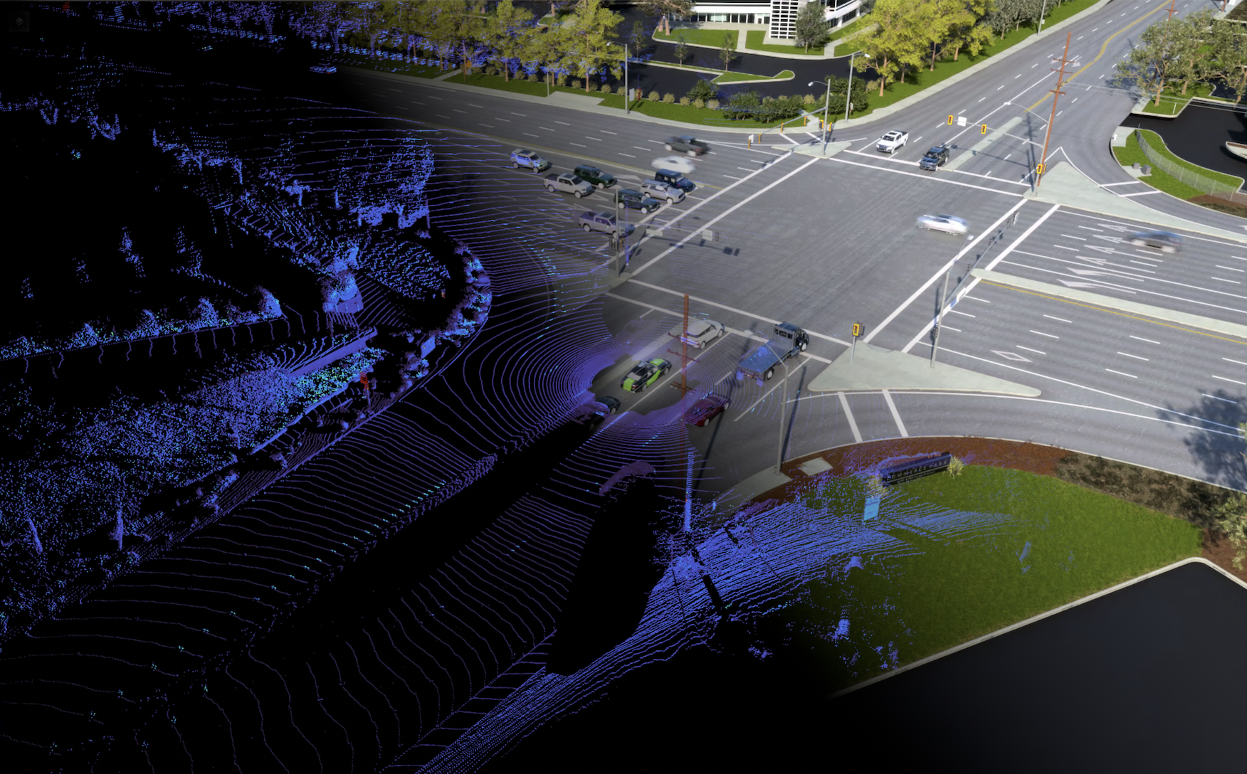
Virtual reconstruction enables developers to find potentially challenging situations to train and validate the AV system with high-fidelity data generated by physically based sensors and AI behavior models that can create many new scenarios. Data from the scenario can also train the behavior model.
Neural Reconstruction
The other approach relies on neural simulation rather than synthetically generating the scene, starting with real sensor data then modifying it.
Sensor replay — the process of playing back recorded sensor data to test the AV system’s performance — is a staple of AV development. This process is open loop, meaning the AV stack’s decisions don’t affect the world since all of the data is prerecorded.
A preview of neural reconstruction methods by NVIDIA Research turn this recorded data into a fully reactive and modifiable world — as in the demo, when the originally recorded van driving past the car could be reenacted to swerve right instead. This revolutionary approach allows closed-loop testing and full interaction between the AV stack and the world it’s driving in.
The process starts with recorded driving data. AI identifies the dynamic objects in the scene and removes them to create an exact replica of the 3D environment that can be rendered from new views. Dynamic objects are then reinserted into the 3D scene with realistic AI-based behaviors and physical appearance, accounting for illumination and shadows.
The AV system then drives in this virtual world and the scene reacts accordingly. The scene can be made more complex through augmented reality by inserting other virtual objects, vehicles and pedestrians which are rendered as if they were part of the real scene and can physically interact with the environment.
Every sensor on the vehicle, including camera and lidar, can be simulated in the scene using AI.
A Virtual World of Possibilities
These new approaches are driven by NVIDIA’s expertise in rendering, graphics and AI.
As a modular platform, DRIVE Sim supports these capabilities with a foundation of deterministic simulation. It provides the vehicle dynamics, AI-based traffic models, scenario tools and a comprehensive SDK to build any tool needed.
With these two powerful new AI methods, developers can easily move from the real world to the virtual one for faster AV development and deployment.
The post NVIDIA Showcases Novel AI Tools in DRIVE Sim to Advance Autonomous Vehicle Development appeared first on NVIDIA Blog.