Surveillance cameras have an identity problem, fueled by an inherent tension between utility and privacy. As these powerful little devices have cropped up seemingly everywhere, the use of machine learning tools has automated video content analysis at a massive scale — but with increasing mass surveillance, there are currently no legally enforceable rules to limit privacy invasions.
Security cameras can do a lot — they’ve become smarter and supremely more competent than their ghosts of grainy pictures past, the ofttimes “hero tool” in crime media. (“See that little blurry blue blob in the right hand corner of that densely populated corner — we got him!”) Now, video surveillance can help health officials measure the fraction of people wearing masks, enable transportation departments to monitor the density and flow of vehicles, bikes, and pedestrians, and provide businesses with a better understanding of shopping behaviors. But why has privacy remained a weak afterthought?
The status quo is to retrofit video with blurred faces or black boxes. Not only does this prevent analysts from asking some genuine queries (e.g., Are people wearing masks?), it also doesn’t always work; the system may miss some faces and leave them unblurred for the world to see. Dissatisfied with this status quo, researchers from MIT’s Computer Science and Artificial Intelligence Laboratory (CSAIL), in collaboration with other institutions, came up with a system to better guarantee privacy in video footage from surveillance cameras. Called “Privid,” the system lets analysts submit video data queries, and adds a little bit of noise (extra data) to the end result to ensure that an individual can’t be identified. The system builds on a formal definition of privacy — “differential privacy” — which allows access to aggregate statistics about private data without revealing personally identifiable information.
Typically, analysts would just have access to the entire video to do whatever they want with it, but Privid makes sure the video isn’t a free buffet. Honest analysts can get access to the information they need, but that access is restrictive enough that malicious analysts can’t do too much with it. To enable this, rather than running the code over the entire video in one shot, Privid breaks the video into small pieces and runs processing code over each chunk. Instead of getting results back from each piece, the segments are aggregated, and that additional noise is added. (There’s also information on the error bound you’re going to get on your result — maybe a 2 percent error margin, given the extra noisy data added).
For example, the code might output the number of people observed in each video chunk, and the aggregation might be the “sum,” to count the total number of people wearing face coverings, or the “average” to estimate the density of crowds.
Privid allows analysts to use their own deep neural networks that are commonplace for video analytics today. This gives analysts the flexibility to ask questions that the designers of Privid did not anticipate. Across a variety of videos and queries, Privid was accurate within 79 to 99 percent of a non-private system.
“We’re at a stage right now where cameras are practically ubiquitous. If there’s a camera on every street corner, every place you go, and if someone could actually process all of those videos in aggregate, you can imagine that entity building a very precise timeline of when and where a person has gone,” says MIT CSAIL PhD student Frank Cangialosi, the lead author on a paper about Privid. “People are already worried about location privacy with GPS — video data in aggregate could capture not only your location history, but also moods, behaviors, and more at each location.”
Privid introduces a new notion of “duration-based privacy,” which decouples the definition of privacy from its enforcement — with obfuscation, if your privacy goal is to protect all people, the enforcement mechanism needs to do some work to find the people to protect, which it may or may not do perfectly. With this mechanism, you don’t need to fully specify everything, and you’re not hiding more information than you need to.
Let’s say we have a video overlooking a street. Two analysts, Alice and Bob, both claim they want to count the number of people that pass by each hour, so they submit a video processing module and ask for a sum aggregation.
The first analyst is the city planning department, which hopes to use this information to understand footfall patterns and plan sidewalks for the city. Their model counts people and outputs this count for each video chunk.
The other analyst is malicious. They hope to identify every time “Charlie” passes by the camera. Their model only looks for Charlie’s face, and outputs a large number if Charlie is present (i.e., the “signal” they’re trying to extract), or zero otherwise. Their hope is that the sum will be non-zero if Charlie was present.
From Privid’s perspective, these two queries look identical. It’s hard to reliably determine what their models might be doing internally, or what the analyst hopes to use the data for. This is where the noise comes in. Privid executes both of the queries, and adds the same amount of noise for each. In the first case, because Alice was counting all people, this noise will only have a small impact on the result, but likely won’t impact the usefulness.
In the second case, since Bob was looking for a specific signal (Charlie was only visible for a few chunks), the noise is enough to prevent them from knowing if Charlie was there or not. If they see a non-zero result, it might be because Charlie was actually there, or because the model outputs “zero,” but the noise made it non-zero. Privid didn’t need to know anything about when or where Charlie appeared, the system just needed to know a rough upper bound on how long Charlie might appear for, which is easier to specify than figuring out the exact locations, which prior methods rely on.
The challenge is determining how much noise to add — Privid wants to add just enough to hide everyone, but not so much that it would be useless for analysts. Adding noise to the data and insisting on queries over time windows means that your result isn’t going to be as accurate as it could be, but the results are still useful while providing better privacy.
Cangialosi wrote the paper with Princeton PhD student Neil Agarwal, MIT CSAIL PhD student Venkat Arun, assistant professor at the University of Chicago Junchen Jiang, assistant professor at Rutgers University and former MIT CSAIL postdoc Srinivas Narayana, associate professor at Rutgers University Anand Sarwate, and assistant professor at Princeton University and Ravi Netravali SM ’15, PhD ’18. Cangialosi will present the paper at the USENIX Symposium on Networked Systems Design and Implementation Conference in April in Renton, Washington.
This work was partially supported by a Sloan Research Fellowship and National Science Foundation grants.
[Summary] tl;dr:
A tremendous amount of effort has been poured into training AI algorithms to competitively play games that computers have traditionally had trouble with, such as the retro games published by Atari, Go, DotA, and StarCraft II. The practical machine learning knowledge accumulated in developing these algorithms has paved the way for people to now routinely train game-playing AI agents for many games. Following this line of work, we focus on a specific category of games – those developed by students as part of a programming assignment. Can the same algorithms that master Atari games help us grade these game assignments? In our recent NeurIPS 2021 paper, we illustrate the challenges in treating interactive coding assignment grading as game playing and introduce the Play to Grade Challenge.
Introduction
Massive Online Coding Education has reached striking success over the past decade. Fast internet speed, improved UI design, code editors that are embedded in a browser window allow educational platforms such as Code.org to build a diverse set of courses tailored towards students of different coding experiences and interest levels (for example, Code.org offers “Star War-themed coding challenge,” and “Elsa/Frozen themed for-loop writing”). As a non-profit organization, Code.org claims to have reached over 60 million learners across the world 1. Such organizations typically provide a variety of carefully constructed teaching materials such as videos and programming challenges.
A challenge faced by these platforms is that of grading assignments. It is well known that grading is critical to student learning 2, in part because it motivates students to complete their assignments. Sometimes manual grading can be feasible in small settings, or automated grading used in simple settings such as when assignments are multiple choice or adopt a fill-in-the-blink modular coding structure. Unfortunately, many of the most exciting assignments, such as developing games or interactive apps, are also much more difficult to automatically evaluate. For such assignments, human teachers are currently needed to provide feedback and grading. This requirement, and the corresponding difficulty with scaling up manual grading, is one of the biggest obstacles of online coding education. Without automated grading systems, students who lack additional teacher resources cannot get useful feedback to help them learn and advance through the materials provided.
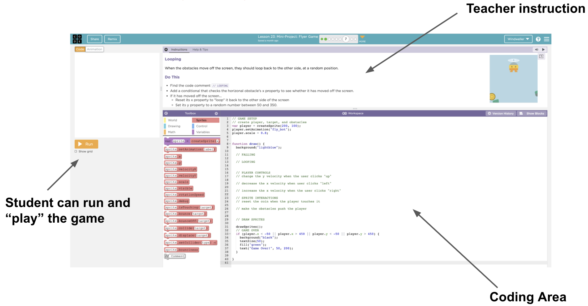
Figure 1: This is a popular coding game offered by Code.org. A student would write a program to create this game.
Programming a game that is playable is exciting for students who are learning to code. Code.org provides many game development assignments in their curriculum. In these assignments, students write JavaScript programs in a code editor embedded in the web browser. Game assignments are great for teachers to examine student’s progress as well: students not only need to grasp basic concepts like if-conditionals and for-loops but use these concepts to write the physical rules of the game world — calculate the trajectories of objects, resolve inelastic collision of two objects, and keep track of game states. To deal with all of these complexities, students need to use abstraction (functions/class) to encapsulate each functionality in order to manage this complex set of logic.
Figure 2: In Code.org, students program in an interactive code interface, where they can write the program in the coding area, hit run and play their game.
Automated grading on the code text alone can be an incredibly hard challenge, even for introductory level computer science assignments. As examples, two solutions which are only slightly different in text can have very different behaviors, and two solutions that are written in very different ways can have the same behaviors. As such, some models that people develop for grading code can be as complex as those used to understand paragraphs of natural language. But, sometimes, grading code can be even more difficult than grading an essay because coding submissions can be in different programming languages. In this situation, one must not only develop a program that can understand many programming languages, but guard against the potential that the grader is more accurate for some languages than others. A Finally, these programs must be able to generalize to new assignments because correct grading is just as necessary for the first student working on an assignment as the millionth – the collect-data, train, deploy cycle is not quite suitable in this context. We don’t have the luxury of collecting a massive amount of labeled dataset to train a fully supervised learning algorithm for each and every assignment.
In a recent paper, we circumvent these challenges by developing a method that grades assignments by playing them, without needing to look at the source code at all. Despite this different approach, our method still manages to provide scalable feedback that potentially can be deployed in a massively-online setting.
The Play to Grade Challenge
Our solution to these problems is to ignore the code text entirely and to grade an assignment by having a grading algorithm play it. We represent the underlying game of each program submission as a Markov Decision Process (MDP), which defines a state space, action space, reward function, and transition dynamics. By running each student’s program, we can build the MDP directly without needing to read or understand the underlying code. You can read more about the MDP framework here: 3.
Since all student programs are written for the same assignment, these programs should generate MDP with a lot of commonalities, such as shared state and action space. After playing the game and fully constructing the MDP for an assignment, all we need is to compare the MDP specified by the student’s program (student MDP) to the teacher’s solution (reference MDP) and determine if these two MDPs are the same. What sets this challenge apart from any other reinforcement learning problems is the fact that a classification needs to be made at the end of this agent’s interaction with this MDP — the decision of whether the MDP is the same as the reference MDP or not.
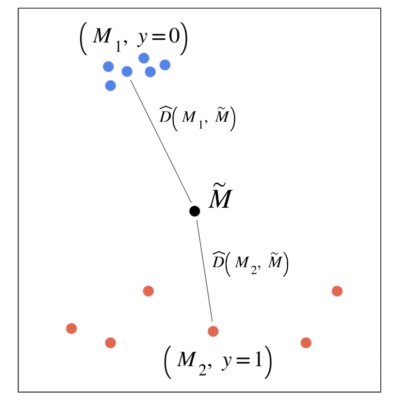
Figure 3: We need to build an approximate distance function D that determines the distance between the student program’s underlying MDP (black dot) and correct MDPs (blue dots) and incorrect MDPs (red dots). Read more about how we build this distance function in our paper.
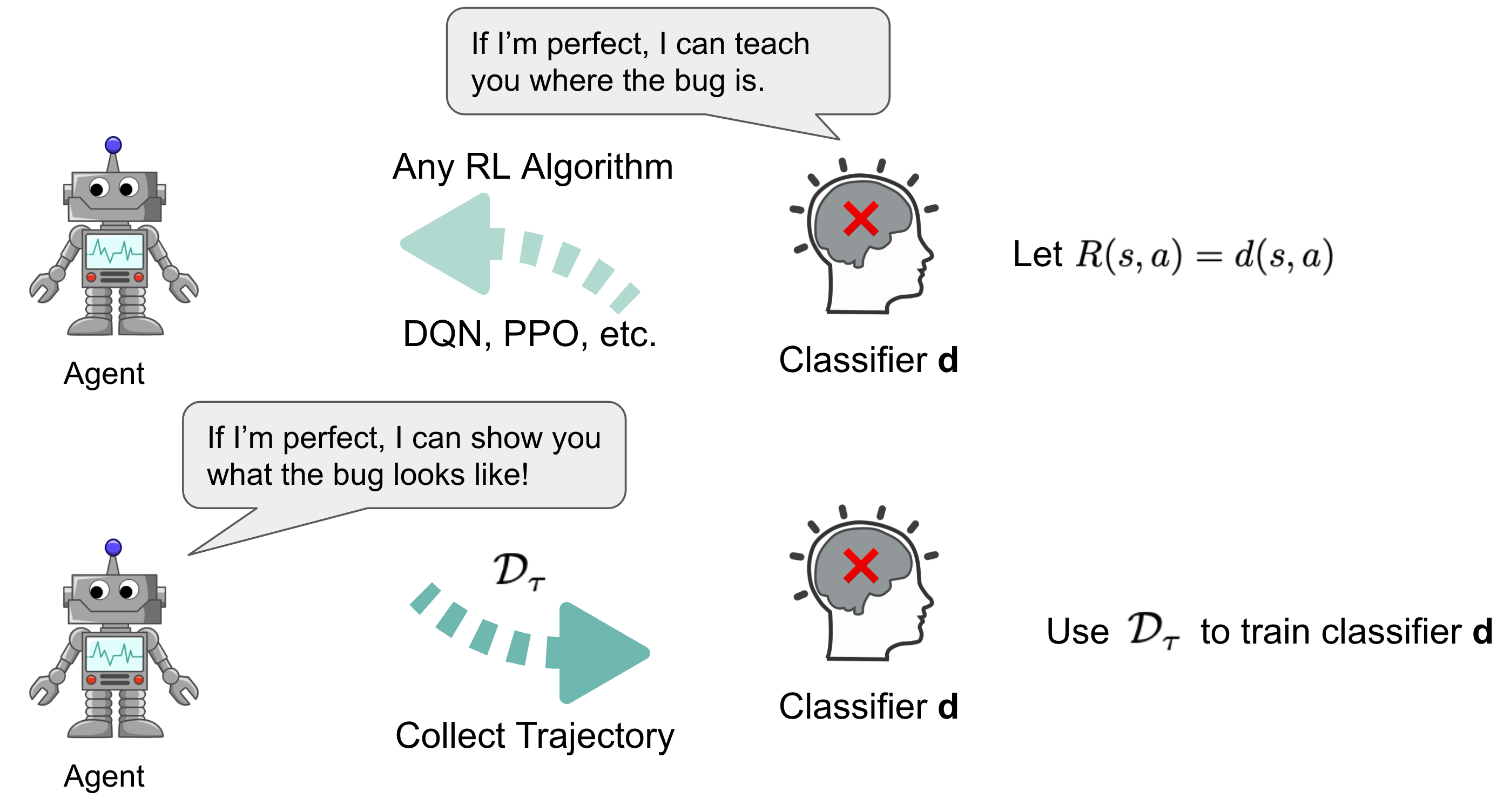
In order to solve this challenge, we present an algorithm with two components: an agent that plays the game and can reliably reach bug states, and a classifier that can recognize bug states (i.e., provide the probability of the observed state being a bug). Both components are necessary for accurate grading: an agent that reaches all states but cannot determine if any represents bugs is just as bad as a perfect classifier paired with an agent that is bad at taking actions which might cause bugs. Imagine a non-optimal agent that never catches the ball (in the example above) – this agent will never be able to test if the wall, or paddle, or goal does not behave correctly.
An ideal agent needs to produce differential trajectories, i.e., sequences of actions that can be used to differentiate two MDPs, and must contain at least one bug-triggering state if the trajectory is produced from the incorrect MDP. Therefore, we need both a correct MDP and a few incorrect MDPs to teach the agent and the classifier. These incorrect MDPs are incorrect solutions that can either be provided by the teacher, or come from manually grading a few student programs to find common issues. Although having to manually label incorrect MDPs is an annoyance, we show that the total amount of effort is generally significantly lower than grading each assignment: in fact, we show that for the task we solve in the paper, you only need 5 incorrect MDPs to reach a decent performance (see the appendix section of our paper).
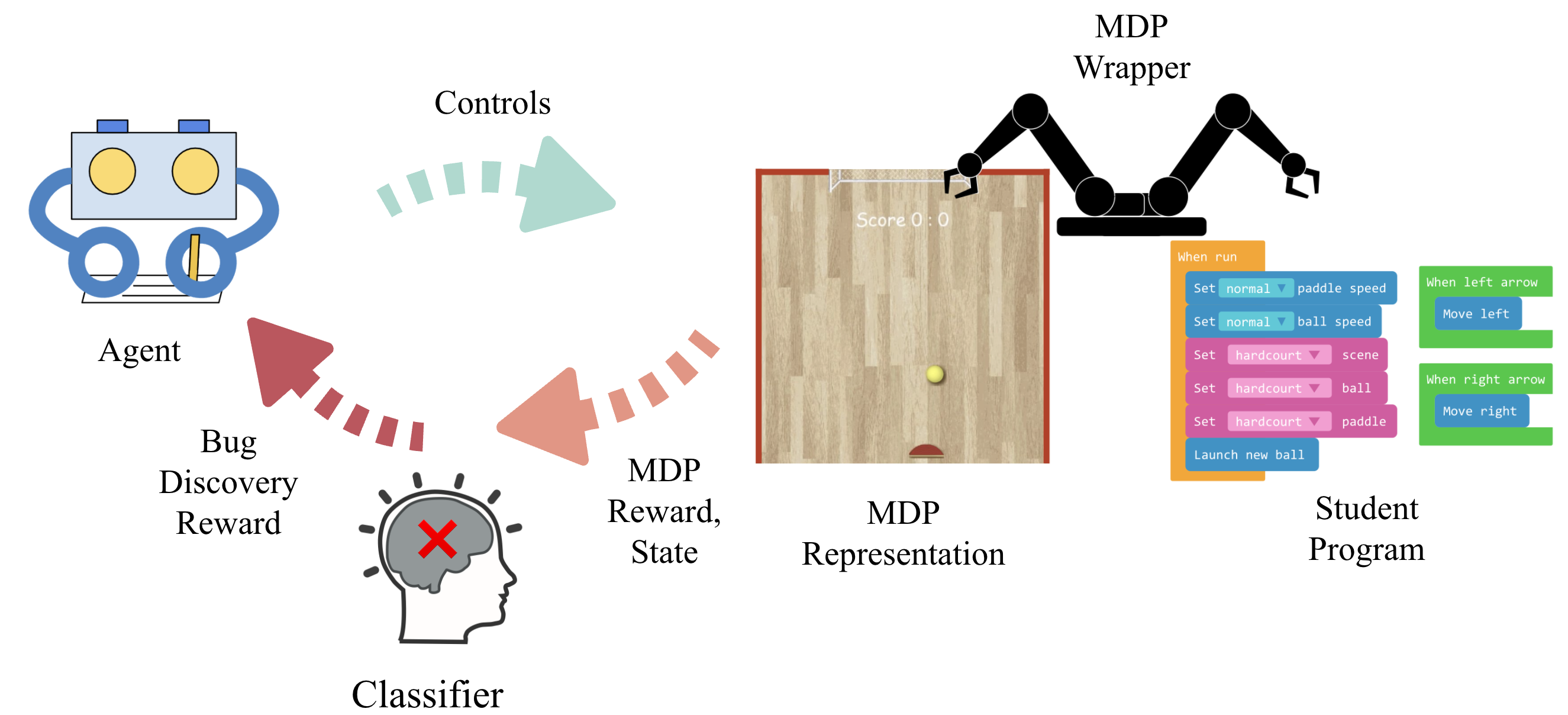
Figure 4: We build an MDP wrapper around the student program that allows the agent to interact with the program (while the original program might only allow human control, i.e., we override mouse / keyboard events.
Recognizing Bugs from Scratch
Here are three incorrect programs and what they look like when played. Each incorrect program behaves differently from the correct program:
One program’s wall does not allow the ball to bounce on it.
Another program’s goal post does not let the ball go through.
The last program spawns 2 new balls whenever the ball bounces on the wall.
Figure 5: Different types of incorrect student programs.
A challenge with building differential trajectories is that one must know which state is a bug triggering state. Previous works 456 have made the strong assumption that one would automatically know when they encountered a bug, potentially because they expect the game program to crash after encountering a bug. Because of this assumption, they focus their efforts on building pure-exploration agents that try to visit as many states as possible. However, in reality, bugs can be difficult to identify and do not all cause the game to crash. For example, a ball that is supposed to bounce off of a wall is now piercing through it and flying off into oblivion. These types of behavioral anomalies motivate the use of a predictive model that can take in the current game state and determine whether it is anomalous or not.
Figure 6: The chicken-and-egg cold-start problem. The agent doesn’t know how to reach bug state, and the classifier does not know what is a bug.
Unfortunately, training a model to predict if a state is a bug state is non-trivial. This is because, although we have labels for some MDPs, these labels are not on the state-level (i.e., not all states in an incorrect MDP are bug states). Put another way, our labels can tell us when a bug has been encountered but cannot tell us what specific action caused the bug. The determination of whether bugs exist in a program can be framed as a chicken-and-egg problem where, if bug states could be unambiguously determined one would only need to explore the state space, and if the exploration was optimal one would only need to figure out how to determine if the current state exhibited a bug.
Collaborative Reinforcement Learning
Fortunately, these types of problems can generally be solved through the expectation-maximization framework, which involves an intimate collaboration between the neural network classifier and the reinforcement learning agent. We propose collaborative reinforcement learning, an expectation-maximization approach, where we use a random agent to produce a dataset of trajectories from the correct and incorrect MDP to teach the classifier. Then the classifier would assign a score to each state indicating how much the classifier believes the state is a bug-triggering state. We use this score as reward and train the agent to reach these states as often as possible for a new dataset of trajectories to train the classifier.
After using the RL agent to interact with the MDP to produce trajectories, we can try out different ways to learn a classifier that can classify a state as a bug or not (a binary label). Choosing the right label is important because this label will become the reward function for the agent, so it can learn to reach bug states more efficiently. However, we only know if the MDP (the submitted code) is correct or broken, but we don’t have labels for the underlying states. Learning state-level labels becomes a challenge!
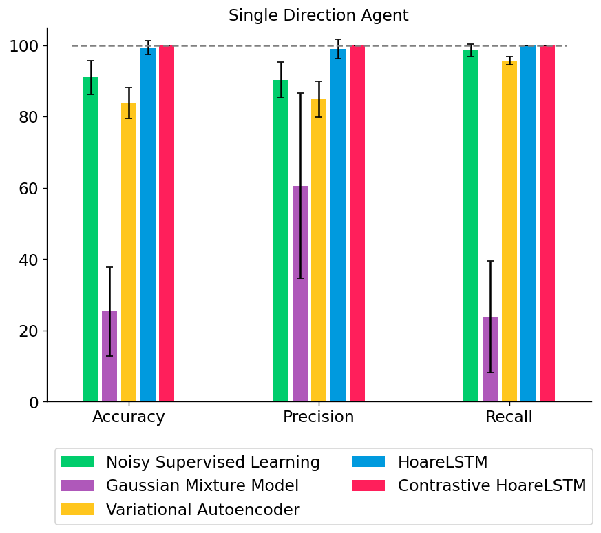
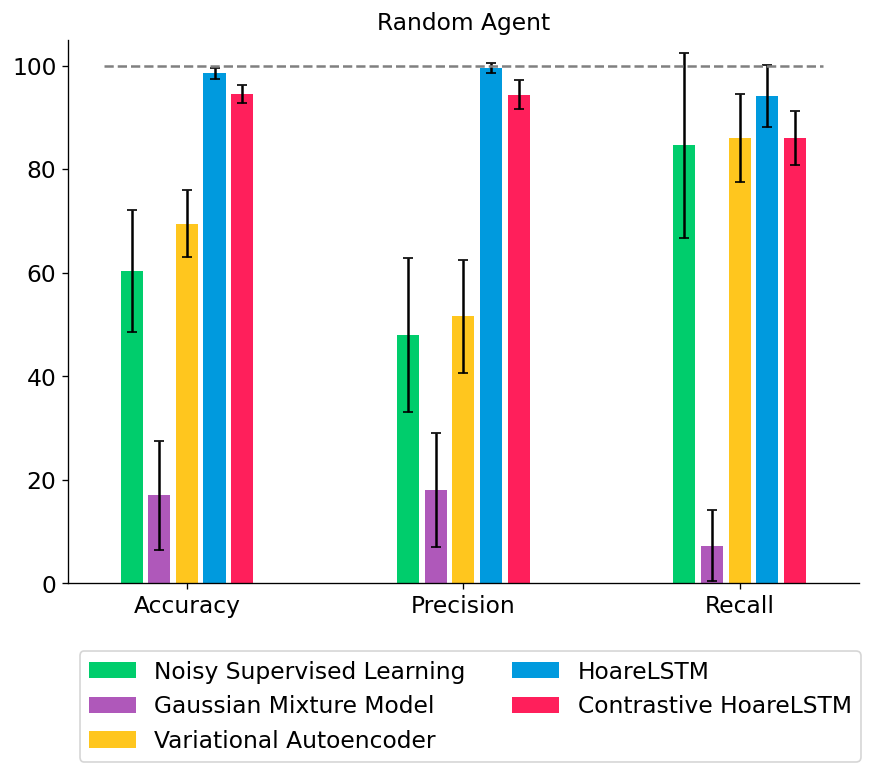
We tested out several types of classifiers: (1) a noisy classifier that classifies all states in a broken MDP as broken, (2) a Gaussian Mixture Model that treats all states independently, (3) a Variational Autoencoder that also treats all states independently but directly models non-linear interactions among the features, or (4) an LSTM that jointly models the teacher program as an MDP (HoareLSTM) and an LSTM that models the student program as an MDP (Contrastive HoareLSTM) – with a distance function that compares the two MDPs, borrowing distance notions from literature in MDP homomorphism78910.
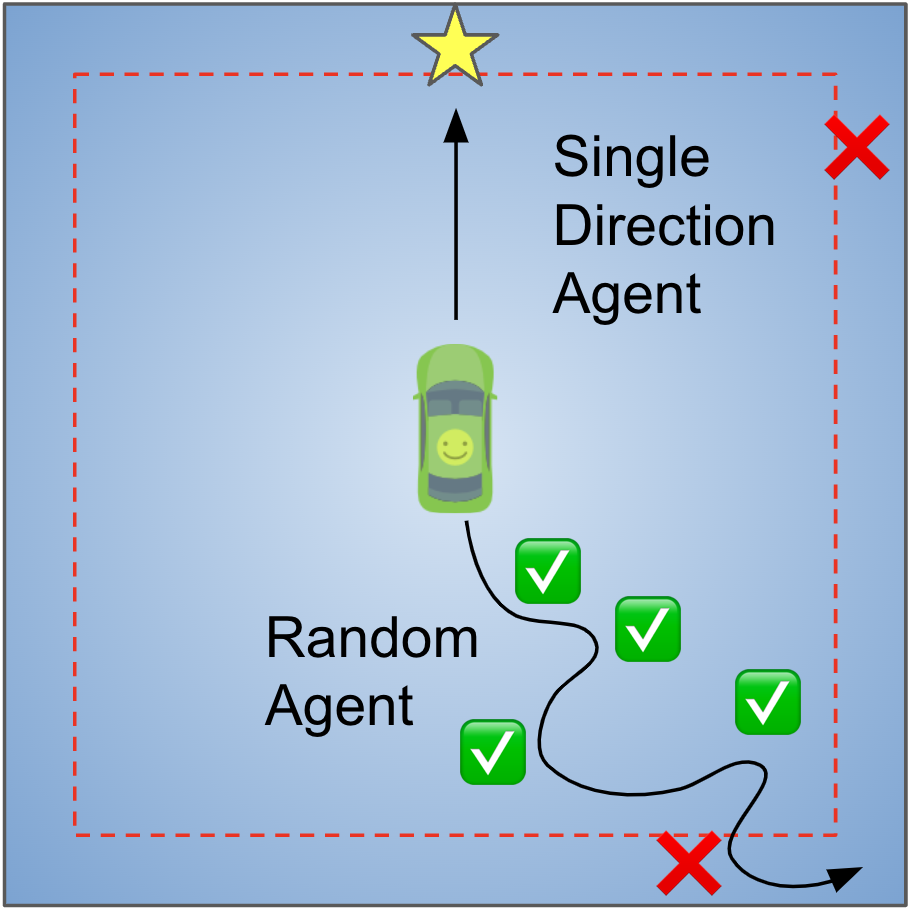
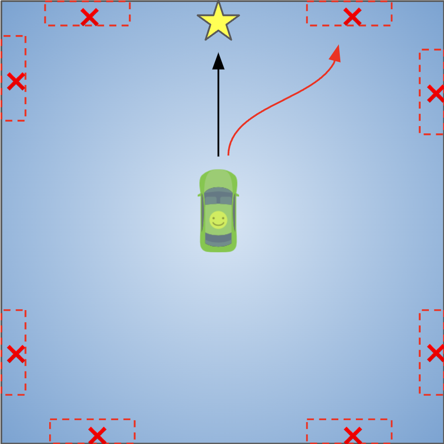
In this toy environment, the agent drives a car on a 2D plane. Whenever the agent drives the car into the outer rim of this area (space between the boundary and red dotted line), a bug will cause the car to get stuck (Leftmost panel in Figure 5). Being stuck means the car’s physical movement is altered, resulting in back-and-forth movement around the same location. The bug classifier needs to recognize the resulting states (position and velocity) of the car being “stuck”, by correctly outputting a binary label (bug) for these states.
In this setting, there is only one type of bug. Most classifiers do well when the agent only drives a straight line (single-direction agent). However, when the agent randomly samples actions at each state, simpler classifiers can no longer differentiate between bug and non-bug states with high accuracy.
Figure 7: Performance of different bug classification models with different RL agents.
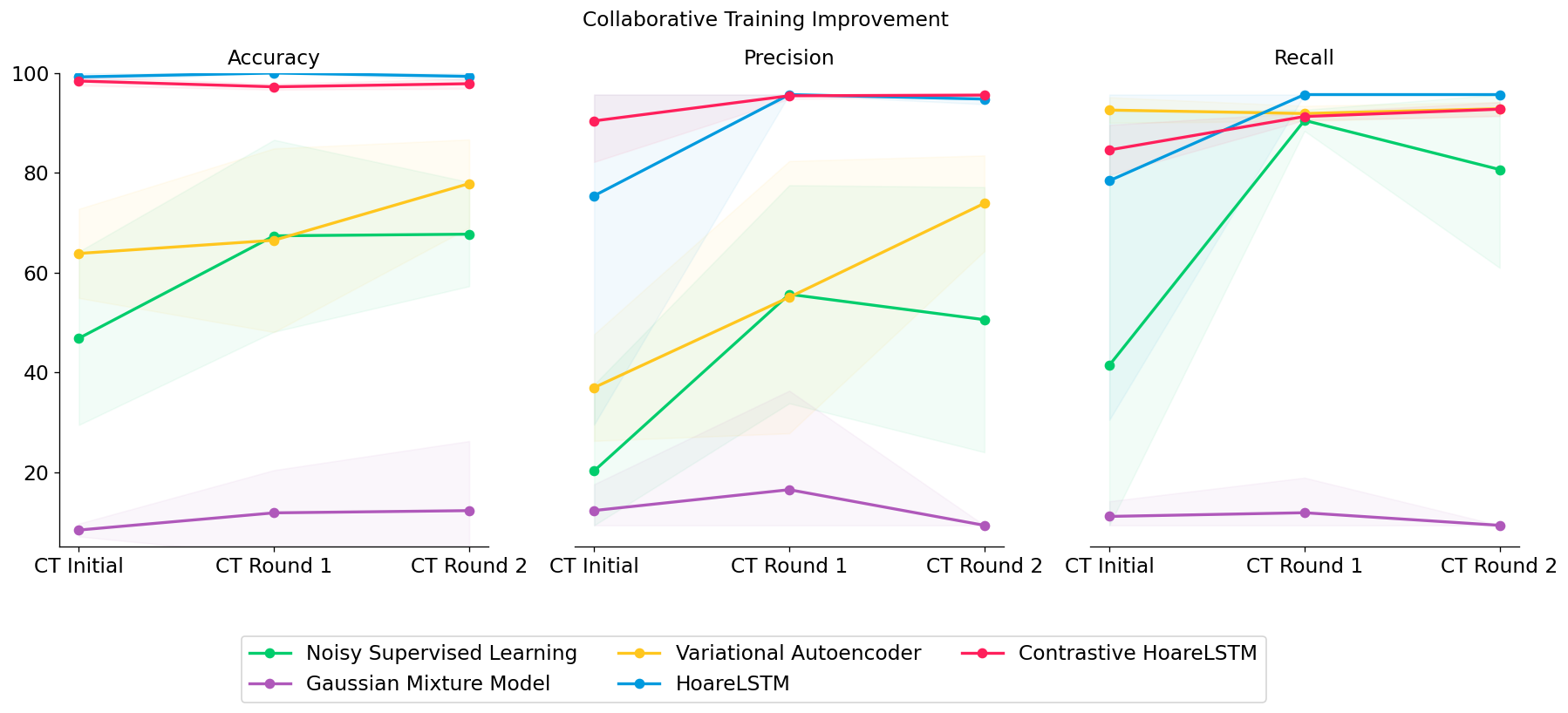
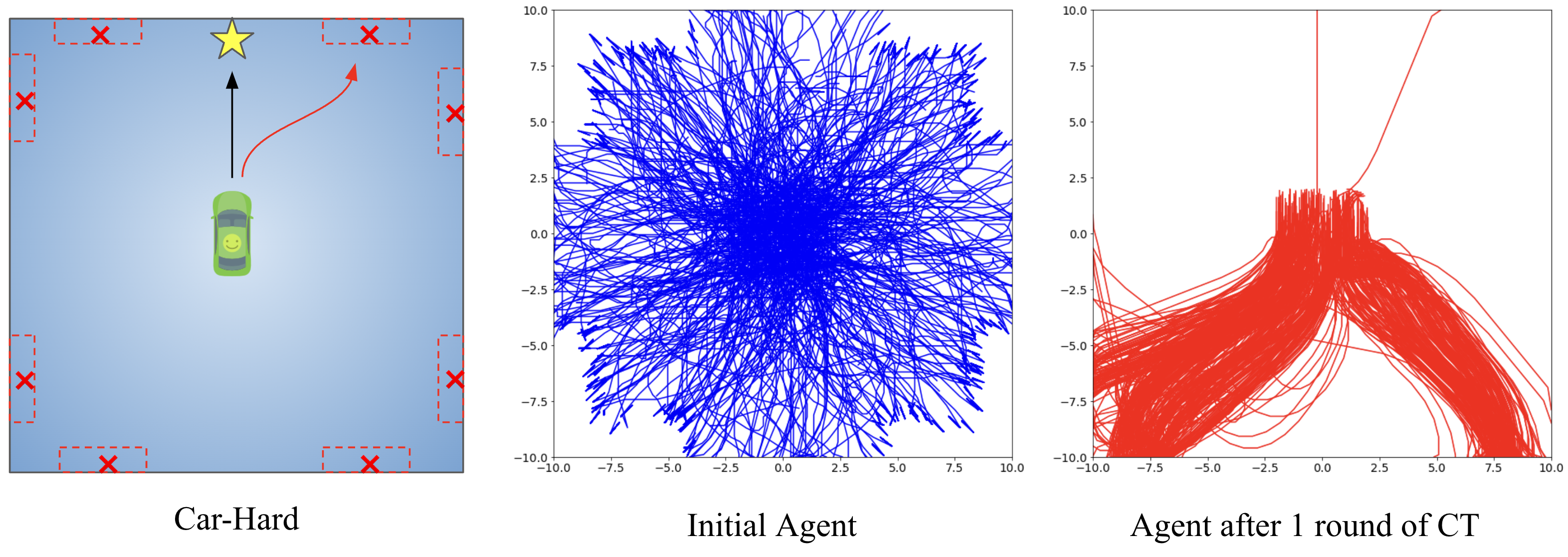
We can increase the difficulty of this setting to see if collaborative training can make the agent operate in the environment with an intention to trigger bugs. In this toy environment, now the bugs will only be triggered in red boxes (Leftmost panel in Figure 6 below). We can see that with only one round of collaborative training (“CT Round 1”), the performances of ALL classifiers are improved, including weaker classifiers. This is understandable, as the agent learns to gradually collect better datasets to train classifiers – and higher quality datasets lead to stronger classifiers. For example, variational auto-encoder started only with 32% precision, but it increased to 74.8% precision after 2 rounds of collaborative training.
Figure 8: Collaborative training improves bug classifier performance across different models. This shows how important it is for the RL agent to produce differential trajectories, which will allow classifiers to obtain higher performance.
We can also visualize how the collaborative training quickly allows the agent to learn to explore states that most-likely contain bugs by visualizing the trajectories (see figure below). Initially the agent just explores the space uniformly (blue curves), but after one round of collaborative training (CT), it learns to focus on visiting the potential bug areas (regions marked by red boxes) (red curves).
Figure 9: Visualization of the paths taken by the RL agent (each line represents one trajectory). After collaborative training (CT), the agent quickly focuses only on visiting potentially bug states (relying on the signal provided by the bug classifiers).
Grading Bounce
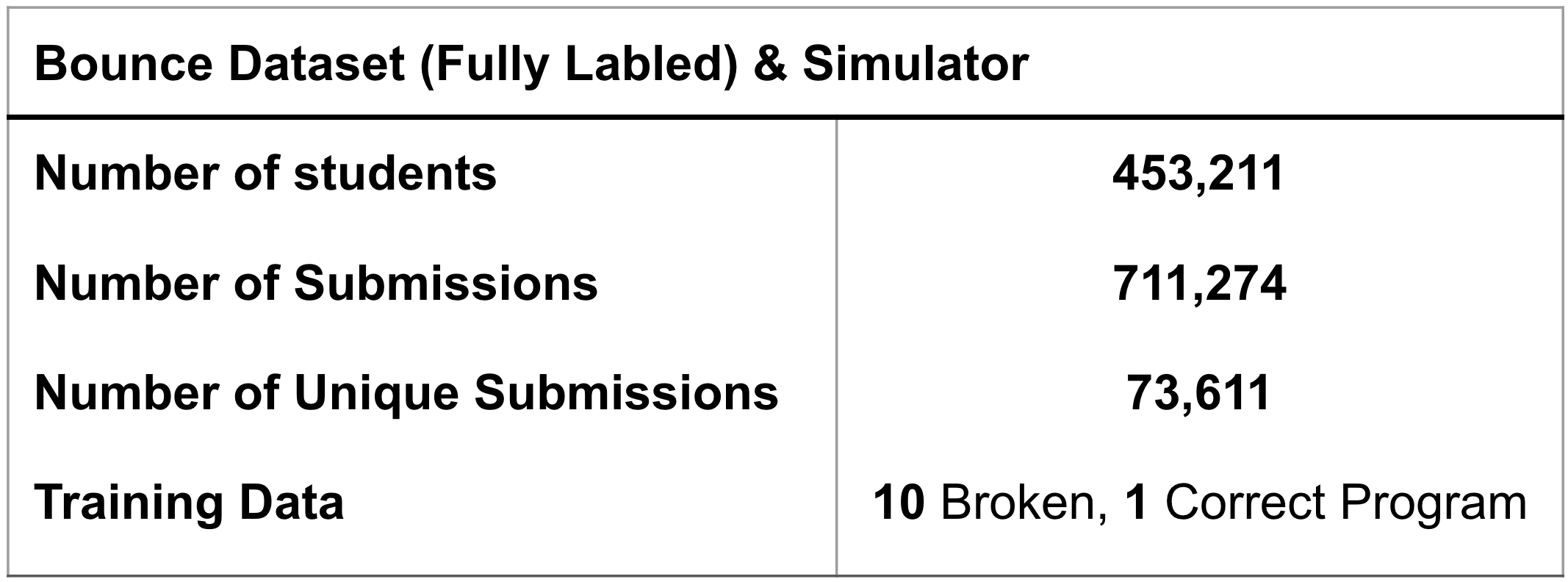
Next, we returned to the motivating example for this type of approach: grading real student submissions. With help from Code.org, we are able to verify the algorithm’s performance on a massive amount of unlabeled, ungraded student submissions. The game Bounce, from Code.org’s Course3 for students in 4th and 5th grade, provides a real-life dataset of what variations of different bugs and behaviors in student programs should look like. The dataset is compiled of 453,211 students who made an attempt on this assignment. In total, this dataset consists of 711,274 programs.
Figure 10: Each program has a binary label (correct or broken) associated with it. We only have 11 programs as our training data.
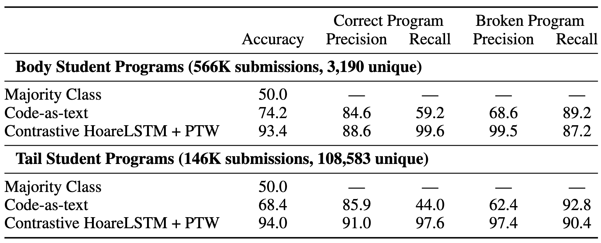
We train our agent and classifier on 10 broken programs that we wrote without looking at any of the student’s submissions. The 10 programs contain bugs that we “guess” to be most likely to occur, and we use them to train 10 agents that learn to reach bug states in these 10 programs. This means that in our training dataset, we have 1 correct program and 10 broken programs. Even with only 11 labeled programs, our agent and classifier can get 99.5% precision at identifying a bug program and 93.4-94% accuracy overall – the agent is able to trigger most of the bugs and the classifier recognizes the bug states using only 10 broken programs. Though for other games, especially more complicated games, the number of training programs will vary. We strongly believe the number is still in magnitude smaller than training supervised code-as-text algorithms. This demonstration shows the promise of reformulating code assignment grading as the Play to Grade.
Figure 11: We show superior performance compared to training a simple code-as-text classifier. For complex, interactive programs, Play to Grade is the most data efficient solution.
What is Next?
We started this project by making the argument that sometimes it is far easier to grade a complex coding assignment not by looking at the code text but by playing it. Using Bounce, we demonstrated that in the simple task of identifying if a program has a bug or not (a binary task, nonetheless), we are able to achieve striking accuracy with only 11 labeled programs. We provide a simulator and all of the student’s programs on this Github repo.
Multi-label Bounce
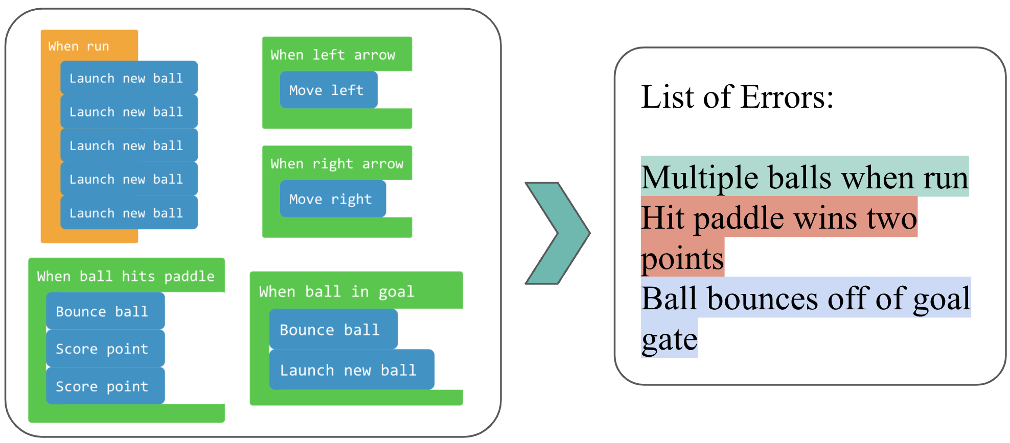
One promising direction for future work is to expand beyond pass/fail binary feedback, and actually identify which bug is in the student’s program and provide that information. Our Bounce dataset enables this by providing multi-error labels, as shown in the table below. The multi-error label setting was not solved by our current algorithm and remains an open challenge!
Figure 12: Each program has a binary label (correct or broken) associated with it. We only have 11 programs as our training data.
More than One Correct Solution
Oftentimes, students create solutions that are creative. Creative solutions are different, but not wrong. For example, students can change the texture pattern of the ball or paddle; or they can make the paddle move much faster. How to set the boundary between “being creative” and “being wrong”? This is not a discussion that happens often in AI, but is of huge importance in education. Though we didn’t use the Bounce dataset to focus on the problem of understanding creativity, our work can still use distance measures to set a “tolerance threshold” to account for creativity.
For Educators
We are interested in collecting a suite of interactive coding assignments and creating a dataset for future researchers to work on this problem. Feel free to reach out to us and let us know what you would consider as important in grading and giving students feedback on their coding assignments!
Conclusion
Providing automated feedback for coding is an important area of research in computational education, and an important area for building fully autonomous coding education pipeline (that can generate coding assignment, grade assignment, and teach interactively). Providing a generalizable algorithm that can play interactive student programs in order to give feedback is an important problem for education and an exciting intellectual challenge for the reinforcement learning community. In this work, we introduce the challenge and a dataset, set up the MDP distance framework that is highly data efficient, algorithms that achieve high accuracy, and demonstrate this is a promising direction of applying machine learning to assist education.
This blog post is based on the following paper:
“Play to Grade: Testing Coding Games as Classifying Markov Decision Process.” Allen Nie, Emma Brunskill, and Chris Piech. Advances in Neural Information Processing Systems 34 (2021). Link
Acknowledgements
Many thanks to Emma Brunskill, Chris Piech for their guidance on the project. Many thanks to Mike Wu, Ali Malik, Yunsung Kim, Lisa Yan, Tong Mu, and Henry Zhu for their discussion and feedback. Special thanks to code.org, and Baker Franke, for many years of collaboration and generously providing the research community with data. Thanks to Stanford Hoffman-Yee Human Centered AI grant for supporting AI in education. Thanks for the numerous rounds of edits from Megha Srivastava and Jacob Schreiber.
Code.org displays this statistics on their landing webpage. ↩
William G Bowen. The ‘cost disease’ in higher education: is technology the answer? The Tanner Lectures Stanford University, 2012. ↩
Gordillo, Camilo, Joakim Bergdahl, Konrad Tollmar, and Linus Gisslén. “Improving Playtesting Coverage via Curiosity Driven Reinforcement Learning Agents.” arXiv preprint arXiv:2103.13798 (2021). ↩
Zhan, Zeping, Batu Aytemiz, and Adam M. Smith. “Taking the scenic route: Automatic exploration for videogames.” arXiv preprint arXiv:1812.03125 (2018). ↩
Zheng, Yan, Xiaofei Xie, Ting Su, Lei Ma, Jianye Hao, Zhaopeng Meng, Yang Liu, Ruimin Shen, Yingfeng Chen, and Changjie Fan. “Wuji: Automatic online combat game testing using evolutionary deep reinforcement learning.” In 2019 34th IEEE/ACM International Conference on Automated Software Engineering (ASE), pp. 772-784. IEEE, 2019. ↩
Pablo Samuel Castro, Prakash Panangaden, and Doina Precup. Equivalence relations in fully and partially observable markov decision processes. In Twenty-First International Joint Conference on Artificial Intelligence, 2009. ↩
Lihong Li, Thomas J Walsh, and Michael L Littman. Towards a unified theory of state abstraction for mdps. ISAIM, 4:5, 2006. ↩
Elise van der Pol, Thomas Kipf, Frans A Oliehoek, and Max Welling. Plannable approximations to mdp homomorphisms: Equivariance under actions. arXiv preprint arXiv:2002.11963, 2020. ↩
Robert Givan, Thomas Dean, and Matthew Greig. Equivalence notions and model minimization in markov decision processes. Artificial Intelligence, 147(1-2):163–223, 2003. ↩
This post is co-written by Shibangi Saha, Data Scientist, and Graciela Kravtzov, Co-Founder and CTO, of Equilibrium Point.
Many individuals are experiencing new symptoms of mental illness, such as stress, anxiety, depression, substance use, and post-traumatic stress disorder (PTSD). According to Kaiser Family Foundation, about half of adults (47%) nationwide have reported negative mental health impacts during the pandemic, a significant increase from pre-pandemic levels. Also, certain genders and age groups are among the most likely to report stress and worry, at rates much higher than others. Additionally, a few specific ethnic groups are more likely to report a “major impact” to their mental health than others.
Several surveys, including those collected by the Centers for Disease Control (CDC), have shown substantial increases in self-reported behavioral health symptoms. According to one CDC report, which surveyed adults across the US in late June of 2020, 31% of respondents reported symptoms of anxiety or depression, 13% reported having started or increased substance use, 26% reported stress-related symptoms, and 11% reported having serious thoughts of suicide in the past 30 days.
Self-reported data, while absolutely critical in diagnosing mental health disorders, can be subject to influences related to the continuing stigma surrounding mental health and mental health treatment. Rather than rely solely on self-reported data, we can estimate and forecast mental distress using data from health records and claims data to try to answer a fundamental question: can we predict who will likely need mental health help before they need it? If these individuals can be identified, early intervention programs and resources can be developed and deployed to respond to any new or increase in underlying symptoms to mitigate the effects and costs of mental disorders.
Easier said than done for those who have struggled with managing and processing large volumes of complex, gap-riddled claims data! In this post, we share how Equilibrium Point IoT used Amazon SageMaker Data Wrangler to streamline claims data preparation for our mental health use case, while ensuring data quality throughout each step in the process.
Solution overview
Data preparation or feature engineering is a tedious process, requiring experienced data scientists and engineers spending a lot of time and energy on formulating recipes for the various transformations (steps) needed to get the data into its right shape. In fact, research shows that data preparation for machine learning (ML) consumes up to 80% of data scientists’ time. Typically, scientists and engineers use various data processing frameworks, such as Pandas, PySpark, and SQL, to code their transformations and create distributed processing jobs. With Data Wrangler, you can automate this process. Data Wrangler is a component of Amazon SageMaker Studio that provides an end-to-end solution to import, prepare, transform, featurize, and analyze data. You can integrate a Data Wrangler data flow into your existing ML workflows to simplify and streamline data processing and feature engineering using little to no coding.
In this post, we walk through the steps to transform original raw datasets into ML-ready features to use for building the prediction models in the next stage. First, we delve into the nature of the various datasets used for our use case and how we joined these datasets via Data Wrangler. After the joins and the dataset consolidation, we describe the individual transformations we applied on the dataset like de-duplication, handling missing values, and custom formulas, followed by how we used the built-in Quick Model analysis to validate the current state of transformations for predictions.
Datasets
For our experiment, we first downloaded patient data from our behavioral health client. This data includes the following:
Claims data
Emergency room visit counts
Inpatient visit counts
Drug prescription counts related to mental health
Hierarchical condition coding (HCC) diagnoses counts related to mental health
The goal was to join these separate datasets based on patient ID and utilize the data to predict a mental health diagnosis. We used Data Wrangler to create a massive dataset of several million rows of data, which is a join of five separate datasets. We also used Data Wrangler to perform several transformations to allow for column calculations. In the following sections, we describe the various data preparation transformations that we applied.
Drop duplicate columns after a join
Amazon SageMaker Data Wrangler provides numerous ML data transforms to streamline cleaning, transforming, and featurizing your data. When you add a transform, it adds a step to the data flow. Each transform you add modifies your dataset and produces a new dataframe. All subsequent transforms apply to the resulting dataframe. Data Wrangler includes built-in transforms, which you can use to transform columns without any code. You can also add custom transformations using PySpark, Pandas, and PySpark SQL. Some transforms operate in place, while others create a new output column in your dataset.
For our experiments, since after each join on the patient ID, we were left with duplicate patient ID columns. We needed to drop these columns. We dropped the right patient ID column, as shown in the following screenshot using the pre-built Manage Columns–>Drop column transform, to maintain only one patient ID column (patient_id in the final dataset).
Pivot a dataset using Pandas
Claims datasets were patient level with emergency visit (ER), inpatient (IP), prescription counts, and diagnoses data already grouped by their correspondent HCC codes (approximately 189 codes). To build a patient datamart, we aggregate the claims HCC codes by patient and pivot the HCC code from rows to columns. We used Pandas to pivot the dataset, count the number of HCC codes by patient, and then join to the primary dataset on patient ID. We used the custom transform option in Data Wrangler choosing Python (Pandas) as the framework of choice.
The following code snippet shows the transformation logic to pivot the table:
# Table is available as variable df
import pandas as pd
import numpy as np

table = pd.pivot_table(df, values = 'claim_count', index=['patient_id0'], columns = 'hcc', fill_value=0).reset_index()
df = table
Create new columns using custom formulas
We studied research literature to determine which HCC codes are deterministic in mental health diagnoses. We then wrote this logic using a Data Wrangler custom formula transform that uses a Spark SQL expression to calculate a Mental Health Diagnosis target column (MH), which we added to the end of the DataFrame.
We used the following transformation logic:
# Output: MH
IF (HCC_Code_11 > 0  or HCC_Code_22 > 0 or HCC_Code_23 > 0   or HCC_Code_54 > 0 or HCC_Code_55 > 0  or HCC_Code_57 > 0    or HCC_Code_72 > 0, 1, 0)
Drop columns from the DataFrame using PySpark
After calculation of the target (MH) column, we dropped all the unnecessary duplicate columns. We preserved the patient ID and the MH column to join to our primary dataset. This was facilitated by a custom SQL transform that uses PySpark SQL as a framework of our choice.
We used the following logic:
/* Table is available as variable df */

select MH, patient_id0 from df
Move the MH column to start
Our ML algorithm requires that the labeled input is in the first column. Therefore, we moved the MH calculated column to the start of the DataFrame to be ready for export.
Fill in blanks with 0 using Pandas
Our ML algorithm also requires that the input data has no empty fields. Therefore, we filled the final dataset’s empty fields with 0s. We can easily do this via a custom transform (Pandas) in Data Wrangler.
We used the following logic:
# Table is available as variable df
df.fillna(0, inplace=True)
Cast column from float to long
You can also parse and cast a column to any new data type easily in Data Wrangler. For memory optimization purposes, we cast our mental health label input column as float.
Quick Model analysis: Feature importance graph
After creating our final dataset, we utilized the Quick Model analysis type in Data Wrangler to quickly identify data inconsistencies and if our model accuracy was in the expected range, or if we needed to continue feature engineering before spending the time of training the model. The model returned an F1 score of 0.901, with 1 being the highest. An F1 score is a way of combining the precision and recall of the model, and it’s defined as the harmonic mean of the two. After inspecting these initial positive results, we were ready to export the data and proceed with model training using the exported dataset.
Export the final dataset to Amazon S3 via a Jupyter notebook
As a final step, to export the dataset in its current form (transformed) to Amazon Simple Storage Service (Amazon S3) for future use on model training, we use the Save to Amazon S3 (via Jupyter Notebook) export option. This notebook starts a distributed and scalable Amazon SageMaker Processing job that applies the created recipe (data flow) to specified inputs (usually larger datasets) and saves the results in Amazon S3. You can also export your transformed columns (features) to Amazon SageMaker Feature Store or export the transformations as a pipeline using Amazon SageMaker Pipelines, or simply export the transformations as Python code.
To export data to Amazon S3, you have three options:
Export the transformed data directly to Amazon S3 via the Data Wrangler UI
Export the transformations as a SageMaker Processing job via a Jupyter notebook (as we do for this post).
Export the transformations to Amazon S3 via a destination node. A destination node tells Data Wrangler where to store the data after you’ve processed it. After you create a destination node, you create a processing job to output the data.
Conclusion
In this post, we showcased how Equilibrium Point IoT uses Data Wrangler to speed up the loading process of large amounts of our claims data for data cleaning and transformation in preparation for ML. We also demonstrated how to incorporate feature engineering with custom transformations using Pandas and PySpark in Data Wrangler, allowing us to export data step by step (after each join) for quality assurance purposes. The application of these easy-to-use transforms in Data Wrangler cut down the time spent on end-to-end data transformation by nearly 50%. Also, the Quick Model analysis feature in Data Wrangler allowed us to easily validate the state of transformations as we cycle through the process of data preparation and feature engineering.
Now that we have prepped the data for our mental health risk modeling use case, as next step, we plan to build an ML model using SageMaker and the built-in algorithms it offers, utilizing our claims dataset to identify members who should seek mental health services before they get to a point where they need it. Stay tuned!
About the Authors
Shibangi Saha is a Data Scientist at Equilibrium Point. She combines her expertise in healthcare payor claims data and machine learning to design, implement, automate, and document for health data pipelines, reporting, and analytics processes that drive insights and actionable improvements in the healthcare delivery system. Shibangi received her Master of Science in Bioinformatics from Northeastern University College of Science and a Bachelor of Science in Biology and Computer Science from Khoury College of Computer Science and Information Sciences.
Graciela Kravtzov is the Co-Founder and CTO of Equilibrium Point. Grace has held C-level/VP leadership positions within Engineering, Operations, and Quality, and served as an executive consultant for business strategy and product development within the healthcare and education industries and the IoT industrial space. Grace received a Master of Science degree in Electromechanical Engineer from the University of Buenos Aires and a Master of Science degree in Computer Science from Boston University.
Arunprasath Shankar is an Artificial Intelligence and Machine Learning (AI/ML) Specialist Solutions Architect with AWS, helping global customers scale their AI solutions effectively and efficiently in the cloud. In his spare time, Arun enjoys watching sci-fi movies and listening to classical music.
Ajai Sharma is a Senior Product Manager for Amazon SageMaker where he focuses on SageMaker Data Wrangler, a visual data preparation tool for data scientists. Prior to AWS, Ajai was a Data Science Expert at McKinsey and Company where he led ML-focused engagements for leading finance and insurance firms worldwide. Ajai is passionate about data science and loves to explore the latest algorithms and machine learning techniques.
Amazon Kendra is an intelligent search service powered by machine learning. You can receive spelling suggestions for misspelled terms in your queries by utilizing the Amazon Kendra Spell Checker. Spell Checker helps reduce the frequency of queries returning irrelevant results by providing spelling suggestions for unrecognized terms.
In this post, we explore how to use Amazon Kendra Spell Checker on the AWS Management Console, as well as how to enable Spell Checker in an Amazon Kendra-powered search application through the AWS Command Line Interface (AWS CLI) and AWS SDK.
Use Amazon Kendra Spell Checker on the console
You can automatically receive spelling suggestions for your misspelled Amazon Kendra queries when querying through the console.
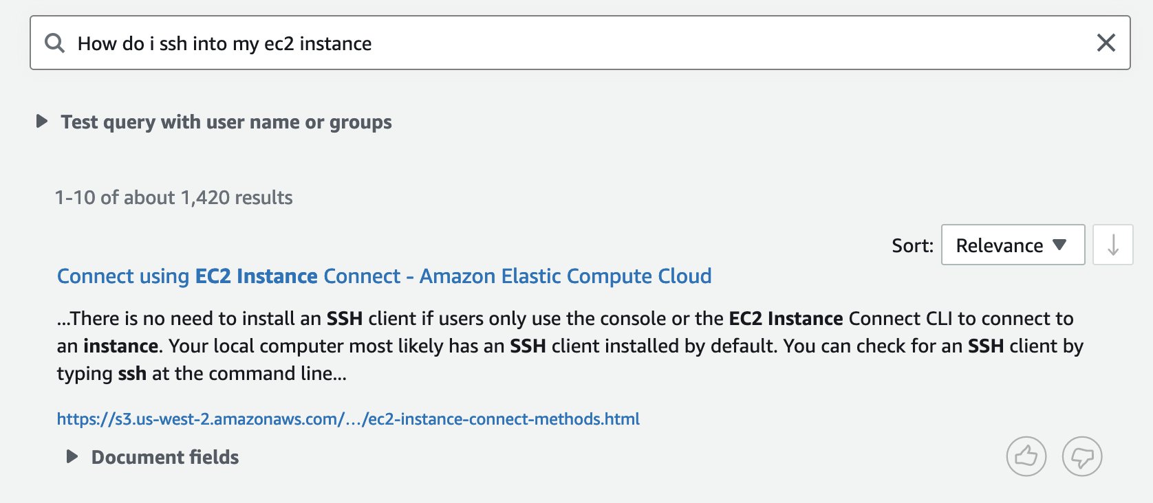
On the Amazon Kendra console, choose your desired index, then choose Search indexed content in the navigation pane. Make sure that the selected index has ingested documents; in this post, we use the sample AWS documentation found in the Data sources section of the navigation pane.
On the Amazon Kendra search console, simply submit a query as you usually would. Misspelled terms in the query are substituted with suggested terms in the “Did you mean” section of the search console.
Choosing the suggested query submits a new query with the corrected spelling.
As you can see, the query results provided through the suggested query are significantly more relevant, thanks to Spell Checker!
Use Amazon Kendra Spell Checker in search applications
Search applications powered by Amazon Kendra can quickly and easily enable Spell Checker through the AWS CLI or AWS SDK, which we walk through in this section. Additionally, we go over an example of how to process the Spell Checker response.
AWS CLI
Let’s look at how AWS CLI users can opt in to Amazon Kendra Spell Checker to receive spelling suggestions for misspelled query terms. We use the AWS CLI to query Amazon Kendra as usual, with only one small change: we include the --spell-correction-configuration IncludeQuerySpellCheckSuggestions=true argument:
In addition to the normal query results, the response from Amazon Kendra now contains a SpellCorrectedQueries object, if there are any spelling suggestions for the query. For more information, see SpellCorrectedQuery.
// Full query response omitted for brevity
"SpellCorrectedQueries": [
  {
    "SuggestedQueryText": "what is kendra",
    "Corrections": [
      {
        "BeginOffset": 8,
        "EndOffset": 14,
        "Term": "knedar",
        "CorrectedTerm": "kendra"
      }
    ]
  }
]
AWS SDK
Next, let’s walk through how Amazon Kendra provides spell check functionality for AWS SDK users. For this example, we use Python 3. We submit a query with a few spelling errors, and print out the SpellCorrectedQueries object in the response:
Now that we’ve gone over how to programmatically get spelling suggestions through either the AWS CLI or AWS SDK, we can examine how we turn the response into a human-readable suggested query. For this example, we use the sample output from the previous section:
Each SpellCorrectedQuery has two keys: SuggestedQueryText and Corrections.
SuggestedQueryText maps to a string containing the updated query with the suggested spelling corrections.
Corrections maps to a list of Correction objects, which contains the beginning and ending offset of the correction, as well as the original term from the query and the spelling suggestion for that term.
For our example, we want to show the suggested query text with the newly suggested terms italicized, similar to what is done on the Amazon Kendra console. To achieve this, we can add HTML italics opening tags <i> at the BeginOffset of each Correction and HTML italics closing tags </i> at the EndOffset of each Correction in the Corrections list. Note that BeginOffset and EndOffset are based on the length of the corrected terms, not the original terms.
Adding the italics tags to SuggestedQueryText gives us the following suggested query text:
kendra <i>free</i> <i>tier</i> hours
As you can see, Amazon Kendra Spell Checker makes it simple to add spell check functionality to your search application.
Conclusion
Spell Checker is a new, powerful feature offered by Amazon Kendra. Spell Checker is a simple, effective way to quickly reduce the number of unhelpful queries by providing spelling suggestions to end-users for misspelled terms.
Spell Checker is available in all AWS Regions where Amazon Kendra is available, and supports all languages currently supported by Amazon Kendra.
Matthew Peretick is a Software Development Engineer at Amazon Web Services based in New York City. Matthew is a member of the Amazon Kendra team focused on enhancing the Amazon Kendra query experience.
If you want to ride the next big wave in AI, grab a transformer.
They’re not the shape-shifting toy robots on TV or the trash-can-sized tubs on telephone poles.
So, What’s a Transformer Model?
A transformer model is a neural network that learns context and thus meaning by tracking relationships in sequential data like the words in this sentence.
Transformer models apply an evolving set of mathematical techniques, called attention or self-attention, to detect subtle ways even distant data elements in a series influence and depend on each other.
First described in a 2017 paper from Google, transformers are among the newest and one of the most powerful classes of models invented to date. They’re driving a wave of advances in machine learning some have dubbed transformer AI.
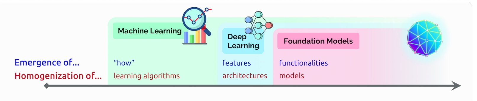
Stanford researchers called transformers “foundation models” in an August 2021 paper because they see them driving a paradigm shift in AI. The “sheer scale and scope of foundation models over the last few years have stretched our imagination of what is possible,” they wrote.
What Can Transformer Models Do?
Transformers are translating text and speech in near real-time, opening meetings and classrooms to diverse and hearing-impaired attendees.
They’re helping researchers understand the chains of genes in DNA and amino acids in proteins in ways that can speed drug design.
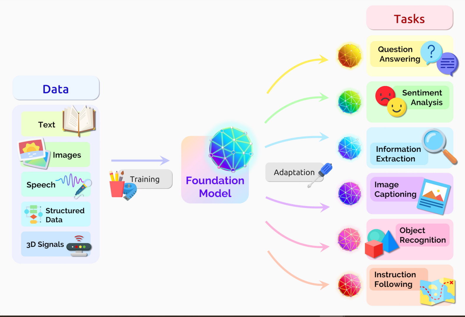
Transformers, sometimes called foundation models, are already being used with many data sources for a host of applications.
Transformers can detect trends and anomalies to prevent fraud, streamline manufacturing, make online recommendations or improve healthcare.
People use transformers every time they search on Google or Microsoft Bing.
The Virtuous Cycle of Transformer AI
Any application using sequential text, image or video data is a candidate for transformer models.
That enables these models to ride a virtuous cycle in transformer AI. Created with large datasets, transformers make accurate predictions that drive their wider use, generating more data that can be used to create even better models.
Stanford researchers say transformers mark the next stage of AI’s development, what some call the era of transformer AI.
“Transformers made self-supervised learning possible, and AI jumped to warp speed,” said NVIDIA founder and CEO Jensen Huang in his keynote address this week at GTC.
Transformers Replace CNNs, RNNs
Transformers are in many cases replacing convolutional and recurrent neural networks (CNNs and RNNs), the most popular types of deep learning models just five years ago.
Indeed, 70 percent of arXiv papers on AI posted in the last two years mention transformers. That’s a radical shift from a 2017 IEEE study that reported RNNs and CNNs were the most popular models for pattern recognition.
No Labels, More Performance
Before transformers arrived, users had to train neural networks with large, labeled datasets that were costly and time-consuming to produce. By finding patterns between elements mathematically, transformers eliminate that need, making available the trillions of images and petabytes of text data on the web and in corporate databases.
In addition, the math that transformers use lends itself to parallel processing, so these models can run fast.
Transformers now dominate popular performance leaderboards like SuperGLUE, a benchmark developed in 2019 for language-processing systems.
How Transformers Pay Attention
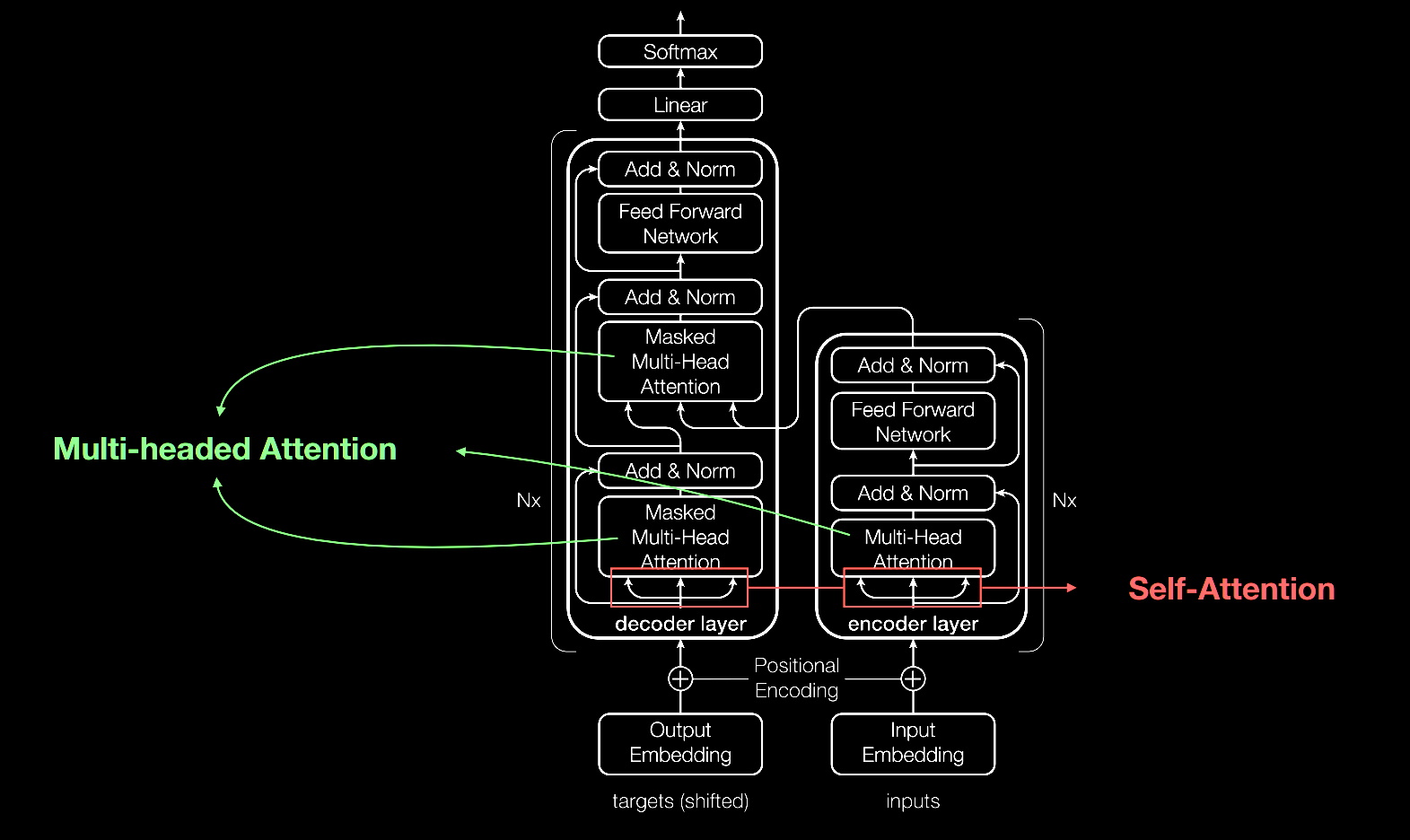
Like most neural networks, transformer models are basically large encoder/decoder blocks that process data.
Small but strategic additions to these blocks (shown in the diagram below) make transformers uniquely powerful.
A look under the hood from a presentation by Aidan Gomez, one of eight co-authors of the 2017 paper that defined transformers.
Transformers use positional encoders to tag data elements coming in and out of the network. Attention units follow these tags, calculating a kind of algebraic map of how each element relates to the others.
Attention queries are typically executed in parallel by calculating a matrix of equations in what’s called multi-headed attention.
With these tools, computers can see the same patterns humans see.
Self-Attention Finds Meaning
For example, in the sentence:
She poured water from the pitcher to the cup until it was full.
We know “it” refers to the cup, while in the sentence:
She poured water from the pitcher to the cup until it was empty.
We know “it” refers to the pitcher.
“Meaning is a result of relationships between things, and self-attention is a general way of learning relationships,” said Ashish Vaswani, a former senior staff research scientist at Google Brain who led work on the seminal 2017 paper.
“Machine translation was a good vehicle to validate self-attention because you needed short- and long-distance relationships among words,” said Vaswani.
“Now we see self-attention is a powerful, flexible tool for learning,” he added.
How Transformers Got Their Name
Attention is so key to transformers the Google researchers almost used the term as the name for their 2017 model. Almost.
“Attention Net didn’t sound very exciting,” said Vaswani, who started working with neural nets in 2011.
.Jakob Uszkoreit, a senior software engineer on the team, came up with the name Transformer.
“I argued we were transforming representations, but that was just playing semantics,” Vaswani said.
The Birth of Transformers
In the paper for the 2017 NeurIPS conference, the Google team described their transformer and the accuracy records it set for machine translation.
Thanks to a basket of techniques, they trained their model in just 3.5 days on eight NVIDIA GPUs, a small fraction of the time and cost of training prior models. They trained it on datasets with up to a billion pairs of words.
“It was an intense three-month sprint to the paper submission date,” recalled Aidan Gomez, a Google intern in 2017 who contributed to the work.
“The night we were submitting, Ashish and I pulled an all-nighter at Google,” he said. “I caught a couple hours sleep in one of the small conference rooms, and I woke up just in time for the submission when someone coming in early to work opened the door and hit my head.”
It was a wakeup call in more ways than one.
“Ashish told me that night he was convinced this was going to be a huge deal, something game changing. I wasn’t convinced, I thought it would be a modest gain on a benchmark, but it turned out he was very right,” said Gomez, now CEO of startup Cohere that’s providing a language processing service based on transformers.
A Moment for Machine Learning
Vaswani recalls the excitement of seeing the results surpass similar work published by a Facebook team using CNNs.
“I could see this would likely be an important moment in machine learning,” he said.
A year later, another Google team tried processing text sequences both forward and backward with a transformer. That helped capture more relationships among words, improving the model’s ability to understand the meaning of a sentence.
Their Bidirectional Encoder Representations from Transformers (BERT) model set 11 new records and became part of the algorithm behind Google search.
Within weeks, researchers around the world were adapting BERT for use cases across many languages and industries “because text is one of the most common data types companies have,” said Anders Arpteg, a 20-year veteran of machine learning research.
Putting Transformers to Work
Soon transformer models were being adapted for science and healthcare.
DeepMind, in London, advanced the understanding of proteins, the building blocks of life, using a transformer called AlphaFold2, described in a recent Nature article. It processed amino acid chains like text strings to set a new watermark for describing how proteins fold, work that could speed drug discovery.
AstraZeneca and NVIDIA developed MegaMolBART, a transformer tailored for drug discovery. It’s a version of pharmaceutical company’s MolBART transformer, trained on a large, unlabeled database of chemical compounds using the NVIDIA Megatron framework for building large-scale transformer models.
Reading Molecules, Medical Records
“Just as AI language models can learn the relationships between words in a sentence, our aim is that neural networks trained on molecular structure data will be able to learn the relationships between atoms in real-world molecules,” said Ola Engkvist, head of molecular AI, discovery sciences and R&D at AstraZeneca, when the work was announced last year.
Separately, the University of Florida’s academic health center collaborated with NVIDIA researchers to create GatorTron. The transformer model aims to extract insights from massive volumes of clinical data to accelerate medical research.
Transformers Grow Up
Along the way, researchers found larger transformers performed better.
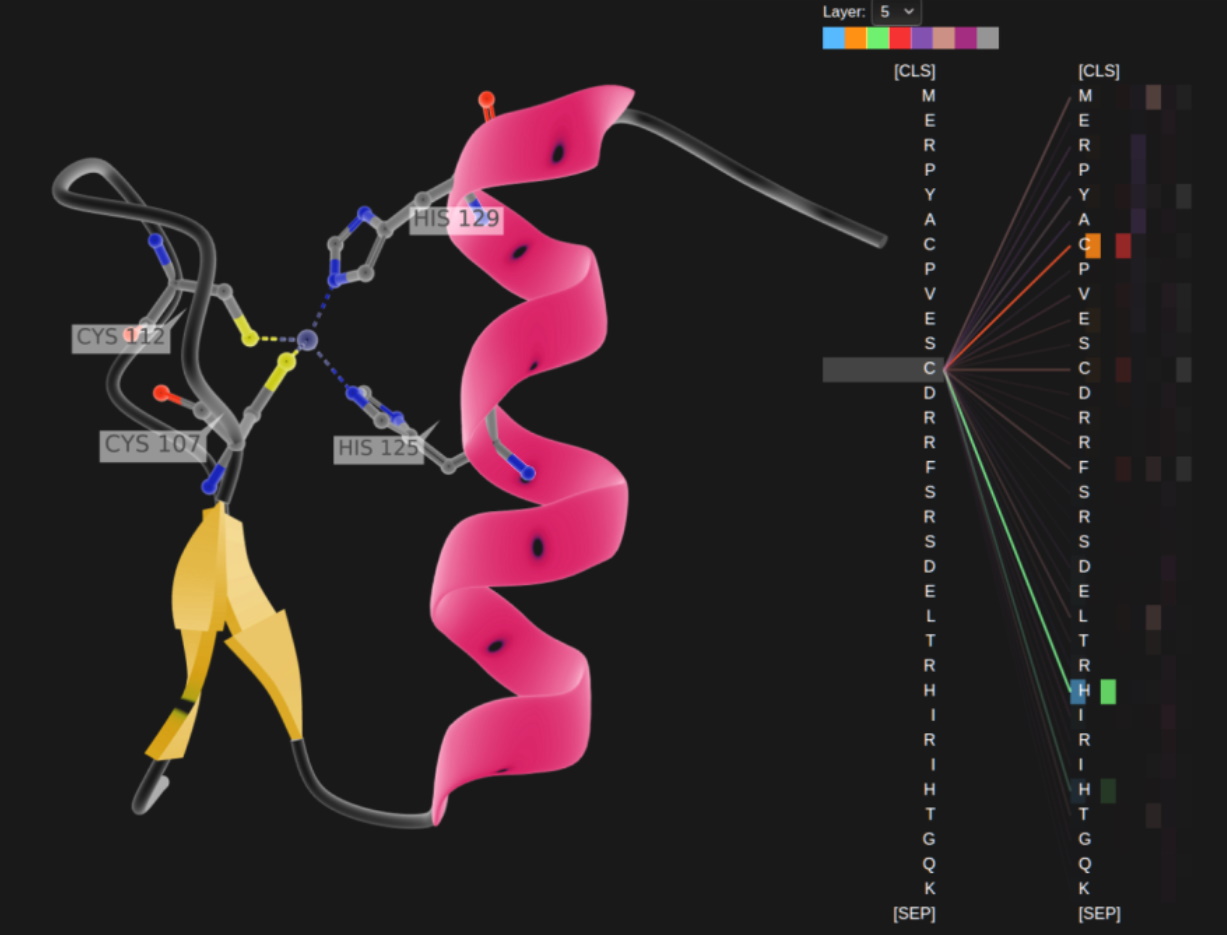
For example, researchers from the Rostlab at the Technical University of Munich, which helped pioneer work at the intersection of AI and biology, used natural-language processing to understand proteins. In 18 months, they graduated from using RNNs with 90 million parameters to transformer models with 567 million parameters.
Rostlab researchers show language models trained without labeled samples picking up the signal of a protein sequence.
The OpenAI lab showed bigger is better with its Generative Pretrained Transformer (GPT). The latest version, GPT-3, has 175 billion parameters, up from 1.5 billion for GPT-2.
With the extra heft, GPT-3 can respond to a user’s query even on tasks it was not specifically trained to handle. It’s already being used by companies including Cisco, IBM and Salesforce.
Tale of a Mega Transformer
NVIDIA and Microsoft hit a high watermark in November, announcing the Megatron-Turing Natural Language Generation model (MT-NLG) with 530 billion parameters. It debuted along with a new framework, NVIDIA NeMo Megatron, that aims to let any business create its own billion- or trillion-parameter transformers to power custom chatbots, personal assistants and other AI applications that understand language.
MT-NLG had its public debut as the brain for TJ, the Toy Jensen avatar that gave part of the keynote at NVIDIA’s November 2021 GTC.
“When we saw TJ answer questions — the power of our work demonstrated by our CEO — that was exciting,” said Mostofa Patwary, who led the NVIDIA team that trained the model.
“Megatron helps me answer all those tough questions Jensen throws at me,” TJ said at GTC 2022.
Creating such models is not for the faint of heart. MT-NLG was trained using hundreds of billions of data elements, a process that required thousands of GPUs running for weeks.
“Training large transformer models is expensive and time-consuming, so if you’re not successful the first or second time, projects might be canceled,” said Patwary.
Trillion-Parameter Transformers
Today, many AI engineers are working on trillion-parameter transformers and applications for them.
“We’re constantly exploring how these big models can deliver better applications. We also investigate in what aspects they fail, so we can build even better and bigger ones,” Patwary said.
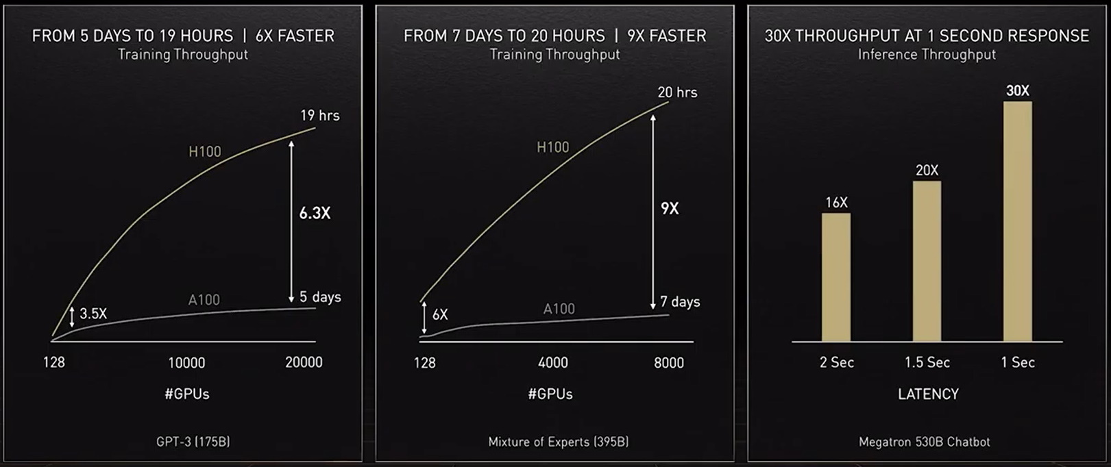
To provide the computing muscle those models need, our latest accelerator — the NVIDIA H100 Tensor Core GPU — packs a Transformer Engine and supports a new FP8 format. That speeds training while preserving accuracy.
With those and other advances, “transformer model training can be reduced from weeks to days” said Huang at GTC.
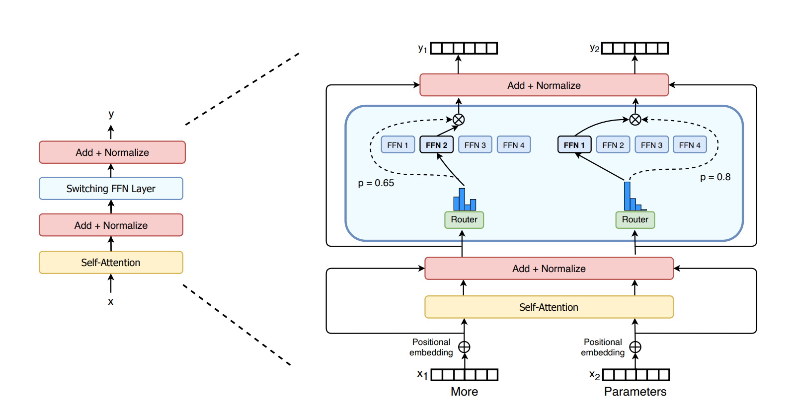
MoE Means More for Transformers
Last year, Google researchers described the Switch Transformer, one of the first trillion-parameter models. It uses AI sparsity, a complex mixture-of experts (MoE) architecture and other advances to drive performance gains in language processing and up to 7x increases in pre-training speed.
The encoder for the Switch Transformer, the first model to have up to a trillion parameters.
Now some researchers aim to develop simpler transformers with fewer parameters that deliver performance similar to the largest models.
“I see promise in retrieval-based models that I’m super excited about because they could bend the curve,” said Gomez, of Cohere, noting the Retro model from DeepMind as an example.
Retrieval-based models learn by submitting queries to a database. “It’s cool because you can be choosy about what you put in that knowledge base,” he said.
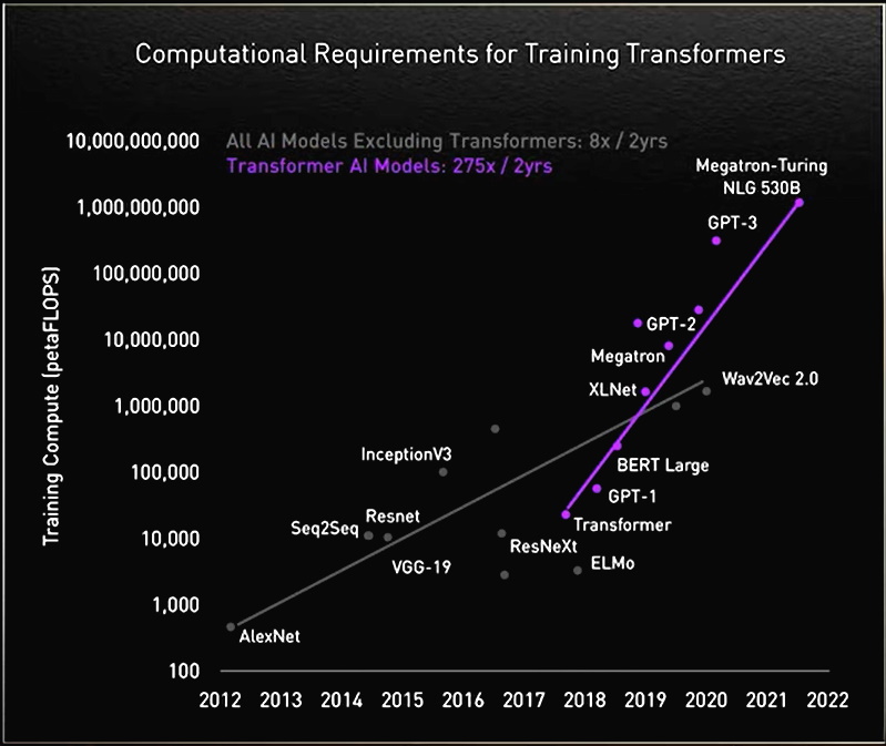
In the race for higher performance, transformer models have grown larger.
The ultimate goal is to “make these models learn like humans do from context in the real world with very little data,” said Vaswani, now co-founder of a stealth AI startup.
He imagines future models that do more computation upfront so they need less data and sport better ways users can give them feedback.
“Our goal is to build models that will help people in their everyday lives,” he said of his new venture.
Safe, Responsible Models
Other researchers are studying ways to eliminate bias or toxicity if models amplify wrong or harmful language. For example, Stanford created the Center for Research on Foundation Models to explore these issues.
“These are important problems that need to be solved for safe deployment of models,” said Shrimai Prabhumoye, a research scientist at NVIDIA who’s among many across the industry working in the area.
“Today, most models look for certain words or phrases, but in real life these issues may come out subtly, so we have to consider the whole context,” added Prabhumoye.
“That’s a primary concern for Cohere, too,” said Gomez. “No one is going to use these models if they hurt people, so it’s table stakes to make the safest and most responsible models.”
Beyond the Horizon
Vaswani imagines a future where self-learning, attention-powered transformers approach the holy grail of AI.
“We have a chance of achieving some of the goals people talked about when they coined the term ‘general artificial intelligence’ and I find that north star very inspiring,” he said.
“We are in a time where simple methods like neural networks are giving us an explosion of new capabilities.”
Transformer training and inference will get significantly accelerated with the NVIDIA H100 GPU.
When the first instant photo was taken 75 years ago with a Polaroid camera, it was groundbreaking to rapidly capture the 3D world in a realistic 2D image. Today, AI researchers are working on the opposite: turning a collection of still images into a digital 3D scene in a matter of seconds.
Known as inverse rendering, the process uses AI to approximate how light behaves in the real world, enabling researchers to reconstruct a 3D scene from a handful of 2D images taken at different angles. The NVIDIA Research team has developed an approach that accomplishes this task almost instantly — making it one of the first models of its kind to combine ultra-fast neural network training and rapid rendering.
NVIDIA applied this approach to a popular new technology called neural radiance fields, or NeRF. The result, dubbed Instant NeRF, is the fastest NeRF technique to date, achieving more than 1,000x speedups in some cases. The model requires just seconds to train on a few dozen still photos — plus data on the camera angles they were taken from — and can then render the resulting 3D scene within tens of milliseconds.
“If traditional 3D representations like polygonal meshes are akin to vector images, NeRFs are like bitmap images: they densely capture the way light radiates from an object or within a scene,” says David Luebke, vice president for graphics research at NVIDIA. “In that sense, Instant NeRF could be as important to 3D as digital cameras and JPEG compression have been to 2D photography — vastly increasing the speed, ease and reach of 3D capture and sharing.”
Showcased in a session at NVIDIA GTC this week, Instant NeRF could be used to create avatars or scenes for virtual worlds, to capture video conference participants and their environments in 3D, or to reconstruct scenes for 3D digital maps.
In a tribute to the early days of Polaroid images, NVIDIA Research recreated an iconic photo of Andy Warhol taking an instant photo, turning it into a 3D scene using Instant NeRF.
What Is a NeRF?
NeRFs use neural networks to represent and render realistic 3D scenes based on an input collection of 2D images.
Collecting data to feed a NeRF is a bit like being a red carpet photographer trying to capture a celebrity’s outfit from every angle — the neural network requires a few dozen images taken from multiple positions around the scene, as well as the camera position of each of those shots.
In a scene that includes people or other moving elements, the quicker these shots are captured, the better. If there’s too much motion during the 2D image capture process, the AI-generated 3D scene will be blurry.
From there, a NeRF essentially fills in the blanks, training a small neural network to reconstruct the scene by predicting the color of light radiating in any direction, from any point in 3D space. The technique can even work around occlusions — when objects seen in some images are blocked by obstructions such as pillars in other images.
Accelerating 1,000x With Instant NeRF
While estimating the depth and appearance of an object based on a partial view is a natural skill for humans, it’s a demanding task for AI.
Creating a 3D scene with traditional methods takes hours or longer, depending on the complexity and resolution of the visualization. Bringing AI into the picture speeds things up. Early NeRF models rendered crisp scenes without artifacts in a few minutes, but still took hours to train.
Instant NeRF, however, cuts rendering time by several orders of magnitude. It relies on a technique developed by NVIDIA called multi-resolution hash grid encoding, which is optimized to run efficiently on NVIDIA GPUs. Using a new input encoding method, researchers can achieve high-quality results using a tiny neural network that runs rapidly.
The model was developed using the NVIDIA CUDA Toolkit and the Tiny CUDA Neural Networks library. Since it’s a lightweight neural network, it can be trained and run on a single NVIDIA GPU — running fastest on cards with NVIDIA Tensor Cores.
The technology could be used to train robots and self-driving cars to understand the size and shape of real-world objects by capturing 2D images or video footage of them. It could also be used in architecture and entertainment to rapidly generate digital representations of real environments that creators can modify and build on.
Beyond NeRFs, NVIDIA researchers are exploring how this input encoding technique might be used to accelerate multiple AI challenges including reinforcement learning, language translation and general-purpose deep learning algorithms.
We reached out to UX Researcher Jose Rodriguez to learn more about his academic and professional background, his journey at Meta so far, and what it’s like to be a UX Researcher at Meta.Read More
A unifying goal of work like this is to develop new disease detection or monitoring approaches that are less invasive, more accurate, cheaper and more readily available. However, one restriction to potential broad population-level applicability of efforts to extract biomarkers from fundus photos is getting the fundus photos themselves, which requires specialized imaging equipment and a trained technician.
The eye can be imaged in multiple ways. A common approach for diabetic retinal disease screening is to examine the posterior segment using fundus photographs (left), which have been shown to contain signals of kidney and heart disease, as well as anemia. Another way is to take photographs of the front of the eye (external eye photos; right), which is typically used to track conditions affecting the eyelids, conjunctiva, cornea, and lens.
In “Detection of signs of disease in external photographs of the eyes via deep learning”, in press at Nature Biomedical Engineering, we show that a deep learning model can extract potentially useful biomarkers from external eye photos (i.e., photos of the front of the eye). In particular, for diabetic patients, the model can predict the presence of diabetic retinal disease, elevated HbA1c (a biomarker of diabetic blood sugar control and outcomes), and elevated blood lipids (a biomarker of cardiovascular risk). External eye photos as an imaging modality are particularly interesting because their use may reduce the need for specialized equipment, opening the door to various avenues of improving the accessibility of health screening.
Developing the Model To develop the model, we used de-identified data from over 145,000 patients from a teleretinal diabetic retinopathy screening program. We trained a convolutional neural network both on these images and on the corresponding ground truth for the variables we wanted the model to predict (i.e., whether the patient has diabetic retinal disease, elevated HbA1c, or elevated lipids) so that the neural network could learn from these examples. After training, the model is able to take external eye photos as input and then output predictions for whether the patient has diabetic retinal disease, or elevated sugars or lipids.
A schematic showing the model generating predictions for an external eye photo.
We measured model performance using the area under the receiver operator characteristic curve (AUC), which quantifies how frequently the model assigns higher scores to patients who are truly positive than patients who are truly negative (i.e., a perfect model scores 100%, compared to 50% for random guesses). The model detected various forms of diabetic retinal disease with AUCs of 71-82%, AUCs of 67-70% for elevated HbA1c, and AUCs of 57-68% for elevated lipids. These results indicate that, though imperfect, external eye photos can help detect and quantify various parameters of systemic health.
Much like the CDC’s pre-diabetes screening questionnaire, external eye photos may be able to help “pre-screen” people and identify those who may benefit from further confirmatory testing. If we sort all patients in our study based on their predicted risk and look at the top 5% of that list, 69% of those patients had HbA1c measurements ≥ 9 (indicating poor blood sugar control for patients with diabetes). For comparison, among patients who are at highest risk according to a risk score based on demographics and years with diabetes, only 55% had HbA1c ≥ 9, and among patients selected at random only 33% had HbA1c ≥ 9.
Assessing Potential Bias We emphasize that this is promising, yet early, proof-of-concept research showcasing a novel discovery. That said, because we believe that it is important to evaluate potential biases in the data and model, we undertook a multi-pronged approach for bias assessment.
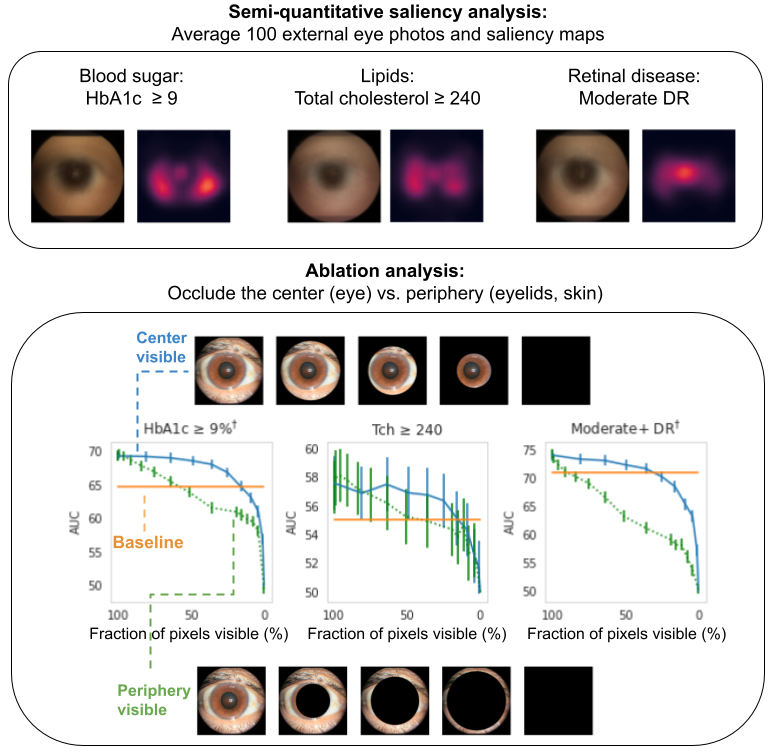
First, we conducted various explainability analyses aimed at discovering what parts of the image contribute most to the algorithm’s predictions (similar to our anemia work). Both saliency analyses (which examine which pixels most influenced the predictions) and ablation experiments (which examine the impact of removing various image regions) indicate that the algorithm is most influenced by the center of the image (the areas of the sclera, iris, and pupil of the eye, but not the eyelids). This is demonstrated below where one can see that the AUC declines much more quickly when image occlusion starts in the center (green lines) than when it starts in the periphery (blue lines).
Explainability analysis shows that (top) all predictions focused on different parts of the eye, and that (bottom) occluding the center of the image (corresponding to parts of the eyeball) has a much greater effect than occluding the periphery (corresponding to the surrounding structures, such as eyelids), as shown by the green line’s steeper decline. The “baseline” is a logistic regression model that takes self-reported age, sex, race and years with diabetes as input.
Second, our development dataset spanned a diverse set of locations within the U.S., encompassing over 300,000 de-identified photos taken at 301 diabetic retinopathy screening sites. Our evaluation datasets comprised over 95,000 images from 198 sites in 18 US states, including datasets of predominantly Hispanic or Latino patients, a dataset of majority Black patients, and a dataset that included patients without diabetes. We conducted extensive subgroup analyses across groups of patients with different demographic and physical characteristics (such as age, sex, race and ethnicity, presence of cataract, pupil size, and even camera type), and controlled for these variables as covariates. The algorithm was more predictive than the baseline in all subgroups after accounting for these factors.
Conclusion This exciting work demonstrates the feasibility of extracting useful health related signals from external eye photographs, and has potential implications for the large and rapidly growing population of patients with diabetes or other chronic diseases. There is a long way to go to achieve broad applicability, for example understanding what level of image quality is needed, generalizing to patients with and without known chronic diseases, and understanding generalization to images taken with different cameras and under a wider variety of conditions, like lighting and environment. In continued partnership with academic and nonacademic experts, including EyePACS and CGMH, we look forward to further developing and testing our algorithm on larger and more comprehensive datasets, and broadening the set of biomarkers recognized (e.g., for liver disease). Ultimately we are working towards making non-invasive health and wellness tools more accessible to everyone.
Acknowledgements This work involved the efforts of a multidisciplinary team of software engineers, researchers, clinicians and cross functional contributors. Key contributors to this project include: Boris Babenko, Akinori Mitani, Ilana Traynis, Naho Kitade, Preeti Singh, April Y. Maa, Jorge Cuadros, Greg S. Corrado, Lily Peng, Dale R. Webster, Avinash Varadarajan, Naama Hammel, and Yun Liu. The authors would also like to acknowledge Huy Doan, Quang Duong, Roy Lee, and the Google Health team for software infrastructure support and data collection. We also thank Tiffany Guo, Mike McConnell, Michael Howell, and Sam Kavusi for their feedback on the manuscript. Last but not least, gratitude goes to the graders who labeled data for the pupil segmentation model, and a special thanks to Tom Small for the ideation and design that inspired the animation used in this blog post.
1The information presented here is research and does not reflect a product that is available for sale. Future availability cannot be guaranteed. ↩
Posted by Raj Pawate (Cadence) and Advait Jain (Google)
Digital Signal Processors (DSPs) are a key part of any battery-powered device offering a way to process audio data with a very low power consumption. These chips run signal processing algorithms such as audio codecs, noise canceling and beam forming.
Increasingly these DSPs are also being used to run neural networks such as wake-word detection, speech recognition, and noise suppression. A key part of enabling such applications is the ability to execute these neural networks as efficiently as possible.
However, productization paths for machine learning on DSPs can often be ad-hoc. In contrast, speech, audio, and video codecs have worldwide standards bodies such as ITU and 3GPP creating algorithms for compression and decompression addressing several aspects of quality measurement, fixed point arithmetic considerations and interoperability.
TensorFlow Lite Micro (TFLM) is a generic open-sourced inference framework that runs machine learning models on embedded targets, including DSPs. Similarly, Cadence has invested heavily in PPA-optimized hardware-software platforms such as Cadence Tensilica HiFi DSP family for audio and Cadence Tensilica Vision DSP family for vision.
Google and Cadence – A Multi-Year Partnership for Enabling AI at the Edge
This was the genesis of the collaboration between the TFLM team and the Audio DSP teams at Cadence, starting in 2019. The TFLM team is focusing on leveraging the broad TensorFlow framework and developing a smooth path from training to embedded and DSP deployment via an interpreter and reference kernels. Cadence is developing a highly optimized software library, called NeuralNet library (NNLIB), that leverages the SIMD and VLIW capabilities of their low-power HiFi DSPs. This collaboration started with three optimized kernels for one Xtensa DSP, and now encompasses over 50 kernels across a variety of platforms such as HiFi 5, HiFi 4, HiFi 3z, Fusion F1 as well as Vision DSPs such as P6, and includes the ability to offload to an accelerator, if available.
Additionally, we have collaborated to add continuous integration for all the optimized code targeted for the Cadence DSPs. This includes infrastructure that tests that every pull request to the TFLM repository passes all the unit tests for the Tensilica toolchain with various HiFix and Vision P6 cores. As such, we ensure that the combined TFLM and NNLIB open source software is both tightly integrated and has good automated test coverage.
Performance Improvements
Most recently, we have collaborated on adding optimizations for models that are quantized with int16 activations. Specifically in the domain of audio, int16 activations can be critical for the quality of quantized generative models. We expect that these optimized kernels will enable a new class of ML-powered audio signal processing. The table below shows a few operators that are required for implementing a noise suppression neural net. We show a 267x improvement in cycle count for a variant of SEANet, an example noise suppression neural net.
The following table shows the improvement with the optimized kernels relative to the reference implementations as measured with the Xtensa instruction set simulation tool.
Operator
Improvement
Transpose Conv
458x
Conv2D
287x
Sub
39x
Add
24x
Leaky ReLU
18x
Srided_Slice
10x
Pad
6x
Overall Network
267x
How to use these optimizations
All of the code can be used from the TFLite Micro GitHub repository.
To use HiFi 3z targeted TFLM optimizations, the following conditions need to be met:
the TensorFlow Lite (TFLite) flatbuffer model is quantized with int16 activations and int8 weights
it uses one or more of the operators listed in the table above
TFLM is compiled with OPTIMIZED_KERNEL_DIR=xtensa
For example, you can run Conv2D kernel integration tests with reference C++ code with:
make -f tensorflow/lite/micro/tools/make/Makefile TARGET=xtensa TARGET_ARCH=hifi4 XTENSA_CORE= test_integration_tests_seanet_conv
And compare that to the optimized kernels by adding OPTIMIZED_KERNEL_DIR=xtensa:
make -f tensorflow/lite/micro/tools/make/Makefile TARGET=xtensa TARGET_ARCH=hifi4 OPTIMIZED_KERNEL_DIR=xtensa XTENSA_CORE= test_integration_tests_seanet_conv
Looking Ahead
While the work thus far has been primarily focused on convolutional neural networks, Google and Cadence are also working together to develop an optimized LSTM operator and have released a first example of an LSTM-based key-word recognizer. We expect to expand on this and continue to bring optimized and production-ready implementations of the latest developments in AI/ML to Tensilica Xtensa DSPs.
Acknowledgements
We would like to acknowledge a number of our colleagues who have contributed to making this collaboration successful.
Google: Advait Jain, Deiqang Chen, Lawrence Chan, Marco Tagliasacchi, Nat Jeffries, Nick Kreeger, Pete Warden, Rocky Rhodes, Ting Yan, Yunpeng Li, Victor Ungureanu