Four professors awarded for research in machine learning and robotics; two doctoral candidates awarded fellowships.Read More

NVIDIA to Reveal New AI Innovations at CES 2024
In the lead-up to next month’s CES trade show in Las Vegas, NVIDIA will unveil its latest advancements in artificial intelligence — including generative AI — and a spectrum of other cutting-edge technologies.
Scheduled for Monday, Jan. 8, at 8 a.m. PT, the company’s special address will be publicly streamed. Save the date and plan to tune in to the virtual address, which will focus on consumer technologies and robotics, on NVIDIA’s website, YouTube or Twitch.
AI and NVIDIA technologies will be the focus of 14 conference sessions, including four at CES Digital Hollywood, “Reshaping Retail – AI Creating Opportunity,” “Robots at Work” and “Cracking the Smart Car.”
And throughout CES, NVIDIA’s story will be enriched by the presence of over 85 NVIDIA customers and partners.
- Consumer: AI, gaming and NVIDIA Studio announcements and demos with partners including Acer, ASUS, Dell, GIGABYTE, HP, Lenovo, MSI, Razer, Samsung, Zotac and more.
- Auto: Showcasing partnerships with leaders including Mercedes-Benz, Hyundai, Kia, Polestar, Luminar and Zoox.
- Robotics: Working alongside Dreame Innovation Technology, DriveU, Ecotron, Enchanted Tools, GluxKind, Hesai Technology, Leopard Imaging, Ninebot (Willand (Beijing) Technology Co., Ltd.), Orbbec, QT Company, Unitree Robotics and Voyant Photonics.
- Enterprise: Collaborations with Accenture, Adobe, Altair, Ansys, AWS, Capgemini, Dassault Systems, Deloitte, Google, Meta, Microsoft, Siemens, Wipro and others.
For the investment community, NVIDIA will participate in a CES Virtual Fireside Chat hosted by J.P. Morgan on Tuesday, Jan. 9, at 8 a.m. PT. Listen to the live audio webcast at investor.nvidia.com.
Visit NVIDIA’s event web page for a complete list of sessions and a view of our extensive partner ecosystem at the show.
Driving advanced analytics outcomes at scale using Amazon SageMaker powered PwC’s Machine Learning Ops Accelerator
This post was written in collaboration with Ankur Goyal and Karthikeyan Chokappa from PwC Australia’s Cloud & Digital business.
Artificial intelligence (AI) and machine learning (ML) are becoming an integral part of systems and processes, enabling decisions in real time, thereby driving top and bottom-line improvements across organizations. However, putting an ML model into production at scale is challenging and requires a set of best practices. Many businesses already have data scientists and ML engineers who can build state-of-the-art models, but taking models to production and maintaining the models at scale remains a challenge. Manual workflows limit ML lifecycle operations to slow down the development process, increase costs, and compromise the quality of the final product.
Machine learning operations (MLOps) applies DevOps principles to ML systems. Just like DevOps combines development and operations for software engineering, MLOps combines ML engineering and IT operations. With the rapid growth in ML systems and in the context of ML engineering, MLOps provides capabilities that are needed to handle the unique complexities of the practical application of ML systems. Overall, ML use cases require a readily available integrated solution to industrialize and streamline the process that takes an ML model from development to production deployment at scale using MLOps.
To address these customer challenges, PwC Australia developed Machine Learning Ops Accelerator as a set of standardized process and technology capabilities to improve the operationalization of AI/ML models that enable cross-functional collaboration across teams throughout ML lifecycle operations. PwC Machine Learning Ops Accelerator, built on top of AWS native services, delivers a fit-for-purpose solution that easily integrates into the ML use cases with ease for customers across all industries. In this post, we focus on building and deploying an ML use case that integrates various lifecycle components of an ML model, enabling continuous integration (CI), continuous delivery (CD), continuous training (CT), and continuous monitoring (CM).
Solution overview
In MLOps, a successful journey from data to ML models to recommendations and predictions in business systems and processes involves several crucial steps. It involves taking the result of an experiment or prototype and turning it into a production system with standard controls, quality, and feedback loops. It’s much more than just automation. It’s about improving organization practices and delivering outcomes that are repeatable and reproducible at scale.
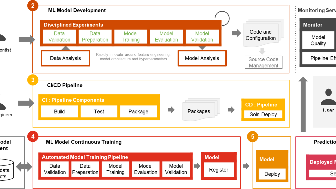
Only a small fraction of a real-world ML use case comprises the model itself. The various components needed to build an integrated advanced ML capability and continuously operate it at scale is shown in Figure 1. As illustrated in the following diagram, PwC MLOps Accelerator comprises seven key integrated capabilities and iterative steps that enable CI, CD, CT, and CM of an ML use case. The solution takes advantage of AWS native features from Amazon SageMaker, building a flexible and extensible framework around this.
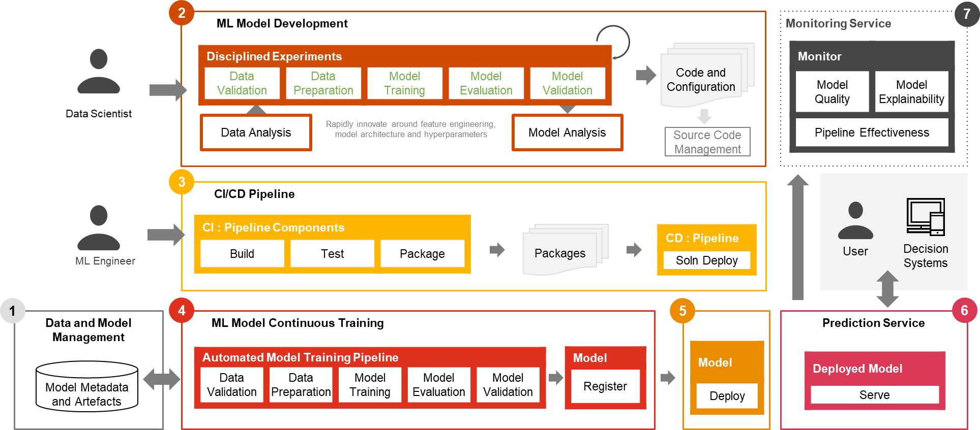
Figure 1 -– PwC Machine Learning Ops Accelerator capabilities
In a real enterprise scenario, additional steps and stages of testing may exist to ensure rigorous validation and deployment of models across different environments.
- Data and model management provide a central capability that governs ML artifacts throughout their lifecycle. It enables auditability, traceability, and compliance. It also promotes the shareability, reusability, and discoverability of ML assets.
- ML model development allows various personas to develop a robust and reproducible model training pipeline, which comprises a sequence of steps, from data validation and transformation to model training and evaluation.
- Continuous integration/delivery facilitates the automated building, testing, and packaging of the model training pipeline and deploying it into the target execution environment. Integrations with CI/CD workflows and data versioning promote MLOps best practices such as governance and monitoring for iterative development and data versioning.
- ML model continuous training capability executes the training pipeline based on retraining triggers; that is, as new data becomes available or model performance decays below a preset threshold. It registers the trained model if it qualifies as a successful model candidate and stores the training artifacts and associated metadata.
- Model deployment allows access to the registered trained model to review and approve for production release and enables model packaging, testing, and deploying into the prediction service environment for production serving.
- Prediction service capability starts the deployed model to provide prediction through online, batch, or streaming patterns. Serving runtime also captures model serving logs for continuous monitoring and improvements.
- Continuous monitoring monitors the model for predictive effectiveness to detect model decay and service effectiveness (latency, pipeline throughout, and execution errors)
PwC Machine Learning Ops Accelerator architecture
The solution is built on top of AWS-native services using Amazon SageMaker and serverless technology to keep performance and scalability high and running costs low.
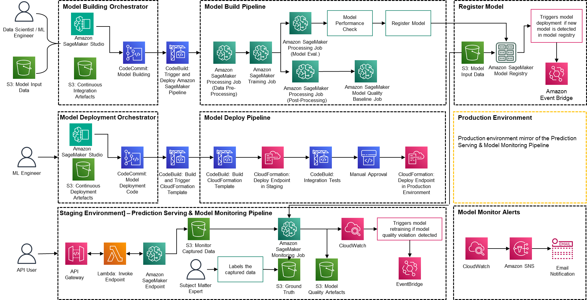
Figure 2 – PwC Machine Learning Ops Accelerator architecture
- PwC Machine Learning Ops Accelerator provides a persona-driven access entitlement for build-out, usage, and operations that enables ML engineers and data scientists to automate deployment of pipelines (training and serving) and rapidly respond to model quality changes. Amazon SageMaker Role Manager is used to implement role-based ML activity, and Amazon S3 is used to store input data and artifacts.
- Solution uses existing model creation assets from the customer and builds a flexible and extensible framework around this using AWS native services. Integrations have been built between Amazon S3, Git, and AWS CodeCommit that allow dataset versioning with minimal future management.
- AWS CloudFormation template is generated using AWS Cloud Development Kit (AWS CDK). AWS CDK provides the ability to manage changes for the complete solution. The automated pipeline includes steps for out-of-the-box model storage and metric tracking.
- PwC MLOps Accelerator is designed to be modular and delivered as infrastructure-as-code (IaC) to allow automatic deployments. The deployment process uses AWS CodeCommit, AWS CodeBuild, AWS CodePipeline, and AWS CloudFormation template. Complete end-to-end solution to operationalize an ML model is available as deployable code.
- Through a series of IaC templates, three distinct components are deployed: model build, model deployment , and model monitoring and prediction serving, using Amazon SageMaker Pipelines
- Model build pipeline automates the model training and evaluation process and enables approval and registration of the trained model.
- Model deployment pipeline provisions the necessary infrastructure to deploy the ML model for batch and real-time inference.
- Model monitoring and prediction serving pipeline deploys the infrastructure required to serve predictions and monitor model performance.
- PwC MLOps Accelerator is designed to be agnostic to ML models, ML frameworks, and runtime environments. The solution allows for the familiar use of programming languages like Python and R, development tools such as Jupyter Notebook, and ML frameworks through a configuration file. This flexibility makes it straightforward for data scientists to continuously refine models and deploy them using their preferred language and environment.
- The solution has built-in integrations to use either pre-built or custom tools to assign the labeling tasks using Amazon SageMaker Ground Truth for training datasets to provide continuous training and monitoring.
- End-to-end ML pipeline is architected using SageMaker native features (Amazon SageMaker Studio , Amazon SageMaker Model Building Pipelines, Amazon SageMaker Experiments, and Amazon SageMaker endpoints).
- The solution uses Amazon SageMaker built-in capabilities for model versioning, model lineage tracking, model sharing, and serverless inference with Amazon SageMaker Model Registry.
- Once the model is in production, the solution continuously monitors the quality of ML models in real time. Amazon SageMaker Model Monitor is used to continuously monitor models in production. Amazon CloudWatch Logs is used to collect log files monitoring the model status, and notifications are sent using Amazon SNS when the quality of the model hits certain thresholds. Native loggers such as (boto3) are used to capture run status to expedite troubleshooting.
Solution walkthrough
The following walkthrough dives into the standard steps to create the MLOps process for a model using PwC MLOps Accelerator. This walkthrough describes a use case of an MLOps engineer who wants to deploy the pipeline for a recently developed ML model using a simple definition/configuration file that is intuitive.
Figure 3 – PwC Machine Learning Ops Accelerator process lifecycle
- To get started, enroll in PwC MLOps Accelerator to get access to solution artifacts. The entire solution is driven from one configuration YAML file (
config.yaml) per model. All the details required to run the solution are contained within that config file and stored along with the model in a Git repository. The configuration file will serve as input to automate workflow steps by externalizing important parameters and settings outside of code. - The ML engineer is required to populate
config.yamlfile and trigger the MLOps pipeline. Customers can configure an AWS account, the repository, the model, the data used, the pipeline name, the training framework, the number of instances to use for training, the inference framework, and any pre- and post-processing steps and several other configurations to check the model quality, bias, and explainability.
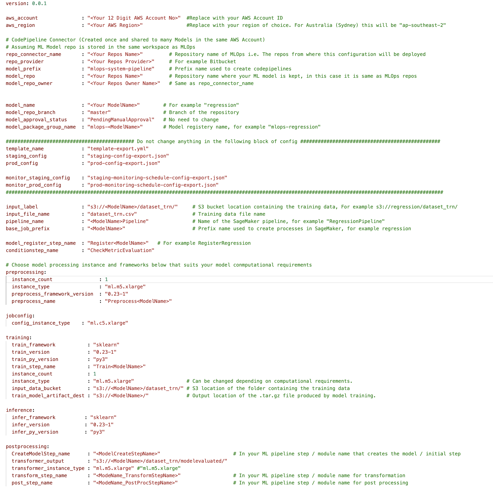
Figure 4 – Machine Learning Ops Accelerator configuration YAML
- A simple YAML file is used to configure each model’s training, deployment, monitoring, and runtime requirements. Once the
config.yamlis configured appropriately and saved alongside the model in its own Git repository, the model-building orchestrator is invoked. It also can read from a Bring-Your-Own-Model that can be configured through YAML to trigger deployment of the model build pipeline. - Everything after this point is automated by the solution and does not need the involvement of either the ML engineer or data scientist. The pipeline responsible for building the ML model includes data preprocessing, model training, model evaluation, and ost-processing. If the model passes automated quality and performance tests, the model is saved to a registry, and artifacts are written to Amazon S3 storage per the definitions in the YAML files. This triggers the creation of the model deployment pipeline for that ML model.
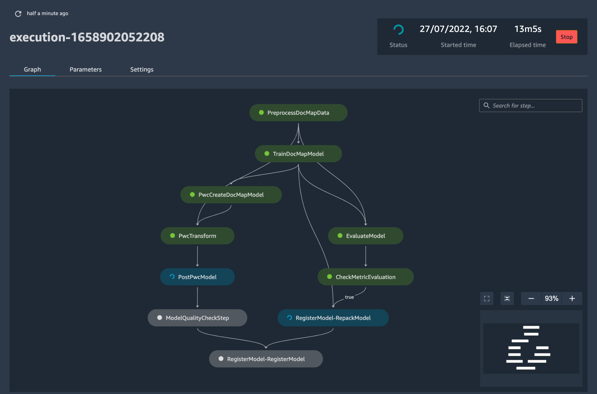
Figure 5 – Sample model deployment workflow
- Next, an automated deployment template provisions the model in a staging environment with a live endpoint. Upon approval, the model is automatically deployed into the production environment.
- The solution deploys two linked pipelines. Prediction serving deploys an accessible live endpoint through which predictions can be served. Model monitoring creates a continuous monitoring tool that calculates key model performance and quality metrics, triggering model retraining if a significant change in model quality is detected.
- Now that you’ve gone through the creation and initial deployment, the MLOps engineer can configure failure alerts to be alerted for issues, for example, when a pipeline fails to do its intended job.
- MLOps is no longer about packaging, testing, and deploying cloud service components similar to a traditional CI/CD deployment; it’s a system that should automatically deploy another service. For example, the model training pipeline automatically deploys the model deployment pipeline to enable prediction service, which in turn enables the model monitoring service.
Conclusion
In summary, MLOps is critical for any organization that aims to deploy ML models in production systems at scale. PwC developed an accelerator to automate building, deploying, and maintaining ML models via integrating DevOps tools into the model development process.
In this post, we explored how the PwC solution is powered by AWS native ML services and helps to adopt MLOps practices so that businesses can speed up their AI journey and gain more value from their ML models. We walked through the steps a user would take to access the PwC Machine Learning Ops Accelerator, run the pipelines, and deploy an ML use case that integrates various lifecycle components of an ML model.
To get started with your MLOps journey on AWS Cloud at scale and run your ML production workloads, enroll in PwC Machine Learning Operations.
About the Authors
 Kiran Kumar Ballari is a Principal Solutions Architect at Amazon Web Services (AWS). He is an evangelist who loves to help customers leverage new technologies and build repeatable industry solutions to solve their problems. He is especially passionate about software engineering , Generative AI and helping companies with AI/ML product development.
 Ankur Goyal is a director in PwC Australia’s Cloud and Digital practice, focused on Data, Analytics & AI. Ankur has extensive experience in supporting public and private sector organizations in driving technology transformations and designing innovative solutions by leveraging data assets and technologies.
 Karthikeyan Chokappa (KC) is a Manager in PwC Australia’s Cloud and Digital practice, focused on Data, Analytics & AI. KC is passionate about designing, developing, and deploying end-to-end analytics solutions that transform data into valuable decision assets to improve performance and utilization and reduce the total cost of ownership for connected and intelligent things.
 Rama Lankalapalli is a Sr. Partner Solutions Architect at AWS, working with PwC to accelerate their clients’ migrations and modernizations into AWS. He works across diverse industries to accelerate their adoption of AWS Cloud. His expertise lies in architecting efficient and scalable cloud solutions, driving innovation and modernization of customer applications by leveraging AWS services, and establishing resilient cloud foundations.
 Jeejee Unwalla is a Senior Solutions Architect at AWS who enjoys guiding customers in solving challenges and thinking strategically. He is passionate about tech and data and enabling innovation.

Simulations illuminate the path to post-event traffic flow

Fifteen minutes. That’s how long it took to empty the Colosseum, an engineering marvel that’s still standing as the largest amphitheater in the world. Two thousand years later, this design continues to work well to move enormous crowds out of sporting and entertainment venues.
But of course, exiting the arena is only the first step. Next, people must navigate the traffic that builds up in the surrounding streets. This is an age-old problem that remains unsolved to this day. In Rome, they addressed the issue by prohibiting private traffic on the street that passes directly by the Colosseum. This policy worked there, but what if you’re not in Rome? What if you’re at the Superbowl? Or at a Taylor Swift concert?
An approach to addressing this problem is to use simulation models, sometimes called “digital twins”, which are virtual replicas of real-world transportation networks that attempt to capture every detail from the layout of streets and intersections to the flow of vehicles. These models allow traffic experts to mitigate congestion, reduce accidents, and improve the experience of drivers, riders, and walkers alike. Previously, our team used these models to quantify sustainability impact of routing, test evacuation plans and show simulated traffic in Maps Immersive View.
Calibrating high-resolution traffic simulations to match the specific dynamics of a particular setting is a longstanding challenge in the field. The availability of aggregate mobility data, detailed Google Maps road network data, advances in transportation science (such as understanding the relationship between segment demands and speeds for road segments with traffic signals), and calibration techniques which make use of speed data in physics-informed traffic models are paving the way for compute-efficient optimization at a global scale.
To test this technology in the real world, Google Research partnered with the Seattle Department of Transportation (SDOT) to develop simulation-based traffic guidance plans. Our goal is to help thousands of attendees of major sports and entertainment events leave the stadium area quickly and safely. The proposed plan reduced average trip travel times by 7 minutes for vehicles leaving the stadium region during large events. We deployed it in collaboration with SDOT using Dynamic Message Signs (DMS) and verified impact over multiple events between August and November, 2023.
 |
 |
| One policy recommendation we made was to divert traffic from S Spokane St, a major thoroughfare that connects the area to highways I-5 and SR 99, and is often congested after events. Suggested changes improved the flow of traffic through highways and arterial streets near the stadium, and reduced the length of vehicle queues that formed behind traffic signals. (Note that vehicles are larger than reality in this clip for demonstration.) |
Simulation model
For this project, we created a new simulation model of the area around Seattle’s stadiums. The intent for this model is to replay each traffic situation for a specified day as closely as possible. We use an open-source simulation software, Simulation of Urban MObility (SUMO). SUMO’s behavioral models help us describe traffic dynamics, for instance, how drivers make decisions, like car-following, lane-changing and speed limit compliance. We also use insights from Google Maps to define the network’s structure and various static segment attributes (e.g., number of lanes, speed limit, presence of traffic lights).
 |
| Overview of the Simulation framework. |
Travel demand is an important simulator input. To compute it, we first decompose the road network of a given metropolitan area into zones, specifically level 13 S2 cells with 1.27 km2 area per cell. From there, we define the travel demand as the expected number of trips that travel from an origin zone to a destination zone in a given time period. The demand is represented as aggregated origin–destination (OD) matrices.
To get the initial expected number of trips between an origin zone and a destination zone, we use aggregated and anonymized mobility statistics. Then we solve the OD calibration problem by combining initial demand with observed traffic statistics, like segment speeds, travel times and vehicular counts, to reproduce event scenarios.
We model the traffic around multiple past events in Seattle’s T-Mobile Park and Lumen Field and evaluate the accuracy by computing aggregated and anonymized traffic statistics. Analyzing these event scenarios helps us understand the effect of different routing policies on congestion in the region.
 |
| Heatmaps demonstrate a substantial increase in numbers of trips in the region after a game as compared to the same time on a non-game day. |
 |
| The graph shows observed segment speeds on the x-axis and simulated speeds on the y-axis for a modeled event. The concentration of data points along the red x=y line demonstrates the ability of the simulation to reproduce realistic traffic conditions. |
Routing policies
SDOT and the Seattle Police Department’s (SPD) local knowledge helped us determine the most congested routes that needed improvement:
- Traffic from T-Mobile Park stadium parking lot’s Edgar Martinez Dr. S exit to eastbound I-5 highway / westbound SR 99 highway
- Traffic through Lumen Field stadium parking lot to northbound Cherry St. I-5 on-ramp
- Traffic going southbound through Seattle’s SODO neighborhood to S Spokane St.
We developed routing policies and evaluated them using the simulation model. To disperse traffic faster, we tried policies that would route northbound/southbound traffic from the nearest ramps to further highway ramps, to shorten the wait times. We also experimented with opening HOV lanes to event traffic, recommending alternate routes (e.g., SR 99), or load sharing between different lanes to get to the nearest stadium ramps.


Evaluation results
We model multiple events with different traffic conditions, event times, and attendee counts. For each policy, the simulation reproduces post-game traffic and reports the travel time for vehicles, from departing the stadium to reaching their destination or leaving the Seattle SODO area. The time savings are computed as the difference of travel time before/after the policy, and are shown in the below table, per policy, for small and large events. We apply each policy to a percentage of traffic, and re-estimate the travel times. Results are shown if 10%, 30%, or 50% of vehicles are affected by a policy.

Based on these simulation results, the feasibility of implementation, and other considerations, SDOT has decided to implement the “Northbound Cherry St ramp” and “Southbound S Spokane St ramp” policies using DMS during large events. The signs suggest drivers take alternative routes to reach their destinations. The combination of these two policies leads to an average of 7 minutes of travel time savings per vehicle, based on rerouting 30% of traffic during large events.
Conclusion
This work demonstrates the power of simulations to model, identify, and quantify the effect of proposed traffic guidance policies. Simulations allow network planners to identify underused segments and evaluate the effects of different routing policies, leading to a better spatial distribution of traffic. The offline modeling and online testing show that our approach can reduce total travel time. Further improvements can be made by adding more traffic management strategies, such as optimizing traffic lights. Simulation models have been historically time consuming and hence affordable only for the largest cities and high stake projects. By investing in more scalable techniques, we hope to bring these models to more cities and use cases around the world.
Acknowledgements
In collaboration with Alex Shashko, Andrew Tomkins, Ashley Carrick, Carolina Osorio, Chao Zhang, Damien Pierce, Iveel Tsogsuren, Sheila de Guia, and Yi-fan Chen. Visual design by John Guilyard. We would like to thank our SDOT partners Carter Danne, Chun Kwan, Ethan Bancroft, Jason Cambridge, Laura Wojcicki, Michael Minor, Mohammed Said, Trevor Partap, and SPD partners Lt. Bryan Clenna and Sgt. Brian Kokesh.

DLSS 3.5 Integration in D5 Render Marks New Era of Real-Time Rendering
Editor’s note: This post is part of our weekly In the NVIDIA Studio series, which celebrates featured artists, offers creative tips and tricks, and demonstrates how NVIDIA Studio technology improves creative workflows.
NVIDIA DLSS 3.5 for realistic ray-traced visuals is now available on D5 Render, a real-time 3D creation software. The integration features DLSS Super Resolution, Frame Generation and Ray Reconstruction powered by an AI neural network.
And this week’s In the NVIDIA Studio 3D artist Michael Gilmour shares his wondrous, intricate winter worlds in long-form videos.
His winter-themed creations join Arkadly Demchenko, Austin Smith and Maggie Shelton’s works in the latest Studio Standouts video, available on the NVIDIA Studio YouTube channel.
Also, tune in to the NVIDIA special address at CES on Jan. 8 at 8 a.m. PT for the latest and greatest on content creation, AI-related news and more.
DLSS 3.5 Accelerates Real-Time Rendering
D5 Render is a software designed for 3D designers and professionals working on large-scale architectural or landscaping projects.

Support for NVIDIA DLSS Frame Generation in D5 Render enhances ray-tracing performance and boosts real-time viewport frame rates for a smoother editing experience, enabling intuitive, interactive 3D creation.

Ray Reconstruction, a new neural rendering AI model, further enhances ray-traced visual quality by providing intelligent denoising solutions for an extensive variety of content at quick speeds.

With both DLSS Frame Generation and Ray Reconstruction enabled, FPS in the viewport increases by a staggering 2.5x, enabling incredible resolution and visual quality in massive scenes.
Autodesk VRED, a professional digital prototyping software, also adds DLSS 3.5 support, bringing smoother viewport movement and higher graphical fidelity.
Winter Tinker
Gilmour, this week’s featured NVIDIA Studio artist, grew up in the beautiful winters of Appleton, Wisconsin. It’s no surprise he conjured up chillingly beautiful winter worlds to share with his friends, family and the creative community — fueled by his passion for 3D art.
Shared as long-form videos, these winter wonderlands showcase breathtakingly photorealistic details.
His winter video compilation — featuring “Campfire on a Winter Cliff,” “Dickensian Christmas Reading Nook” and “Northern Lights” — is designed to offer viewers a sense of peace and relaxation while encouraging self-reflection.
Gilmour began his creative workflows in Unreal Engine, building out the environments. He used the Ultra Dynamic Sky system plug-in by game developer Everett Gunther, which offered greater flexibility and more customization options to achieve the effects in this northern lights scene.
Fully built models are available in Unreal Engine, but to achieve further customization, Gilmour created custom 3D meshes in Blender. He used Blender Cycles’ NVIDIA RTX-accelerated OptiX ray tracing in the viewport for interactive, photorealistic rendering — all powered by his GeForce RTX 3060 graphics card.
“Originally, I chose an NVIDIA RTX GPU because of its CUDA core integration in Blender’s Cycles rendering engine,” said Gilmour. “Now with ray-tracing capabilities in Unreal Engine 5, it’s a no-brainer.”

He then acquired models in Quixel Megascans to block out the scene in Unreal Engine, creating a rough draft using simple, unpolished 3D shapes. This helped to keep base meshes clean, eliminating the need to create new ones in the next iteration.

To build the fire and glowing firewood in his “Campfire on a Winter Cliff” scene, Gilmour used the M5 VFX Vol 2 and Twinmotion Backyard Pack 2 packs from Unreal Engine. The NVIDIA PhysX SDK, advanced shader support and real-time ray tracing enabled high-fidelity, interactive visualization for swift viewport movement.
By upgrading to a GeForce RTX 40 Series GPU, Gilmour could use NVIDIA DLSS Frame Generation to further improve viewport interactivity by tapping AI to generate additional, high-quality frames, ensuring increased FPS rendered at lower resolution while retaining high-fidelity detail.
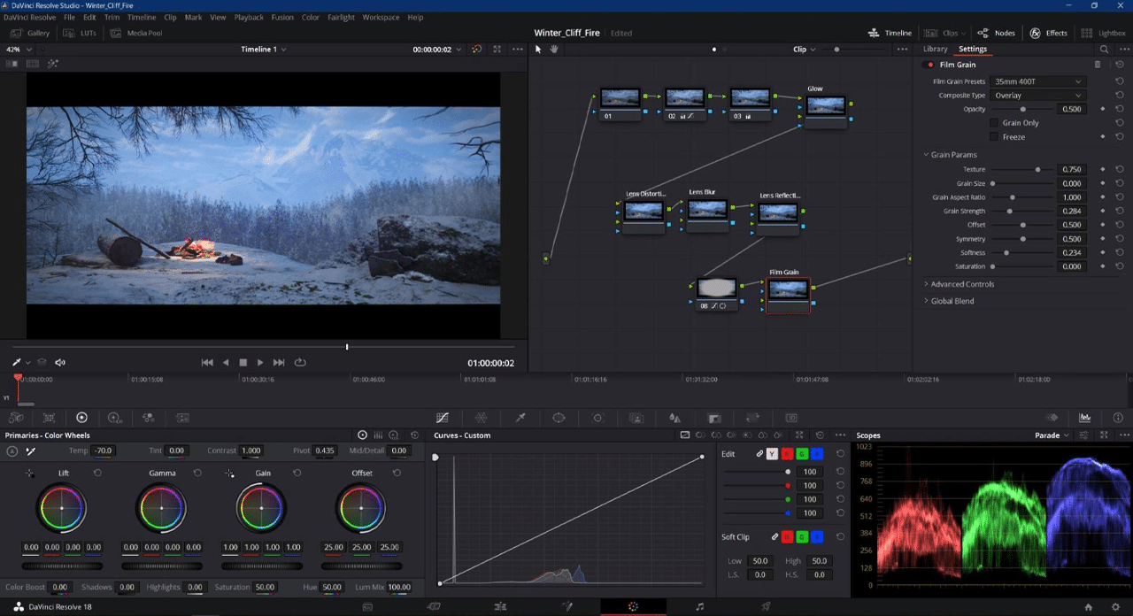
When finished building his scenes, Gilmour moved to Blackmagic Design’s DaVinci Resolve to color correct and add subtle film grains, lens distortion, lens reflection and glow effects. It was all GPU-accelerated, including the process of exporting final videos with the eighth-generation NVENC encoder.
The final touch to Gilmour’s wintry scenes were peaceful tunes, sampled from royalty-free music database Splice.
All that’s left to do is kick back, relax and soak in the scenery.

Check out Gilmour’s portfolio on ArtStation.
Follow NVIDIA Studio on Instagram, Twitter and Facebook. Access tutorials on the Studio YouTube channel and get updates directly in your inbox by subscribing to the Studio newsletter.
Understanding GPU Memory 2: Finding and Removing Reference Cycles
This is part 2 of the Understanding GPU Memory blog series. Our first post Understanding GPU Memory 1: Visualizing All Allocations over Time shows how to use the memory snapshot tool. In this part, we will use the Memory Snapshot to visualize a GPU memory leak caused by reference cycles, and then locate and remove them in our code using the Reference Cycle Detector.
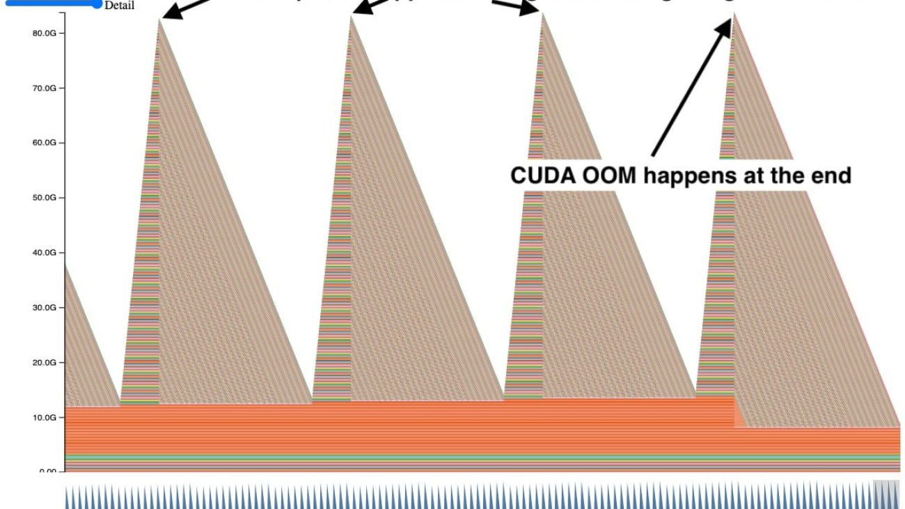
Sometimes when we were using the Memory Snapshot, we saw plots of GPU memory that looked similar to this.
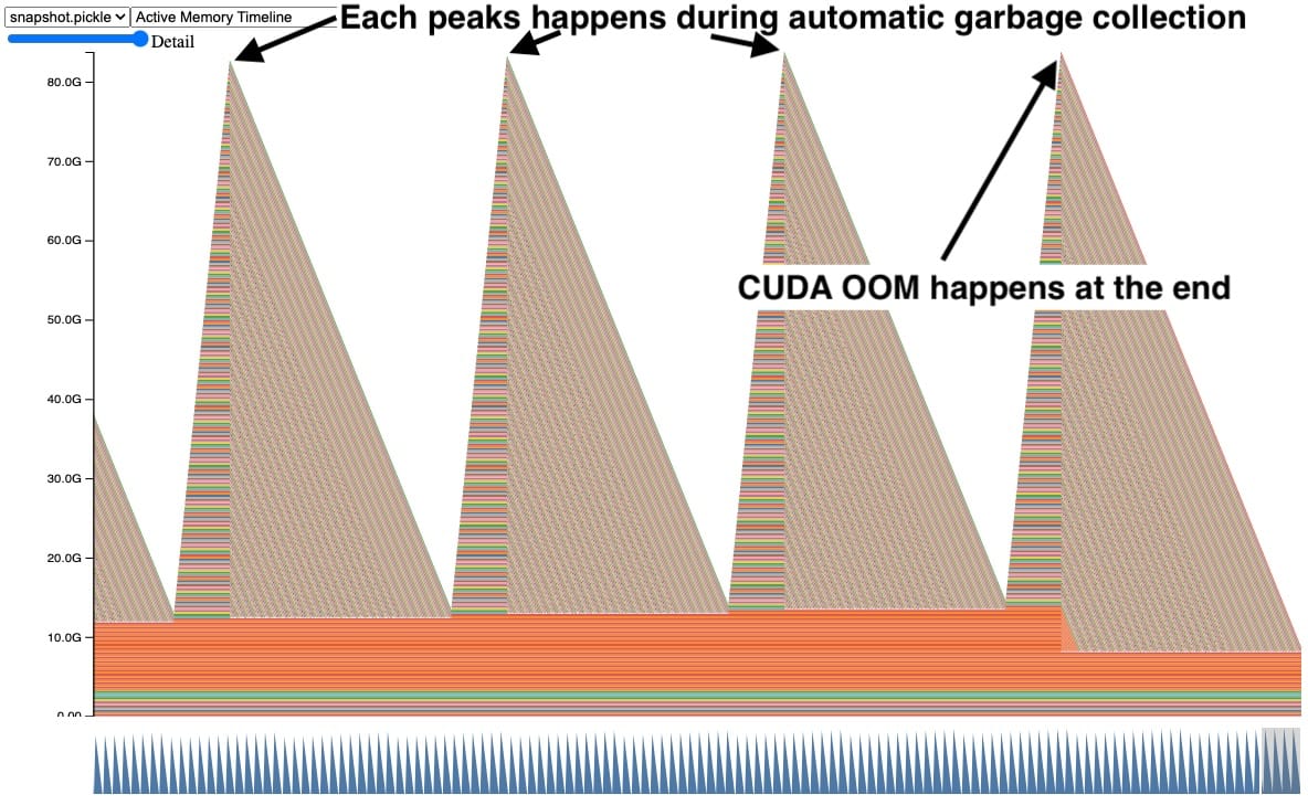
In this snapshot, each peak shows GPU tensors building up over time and then several tensors getting released at once. In addition, a CUDA OOM happens on the right side causing all the tensors to be released. Seeing the tensors accumulate like this is a clear indication of a problem, but it doesn’t immediately suggest why.
Tensors in Reference Cycles
During early debugging, we dug in further to find that this **pattern happens a lot when your Python code has objects with reference cycles. ** Python will clean up non-cyclic objects immediately using reference counting. However objects in reference cycles are only cleaned up later by a cycle collector. If these cycles refer to a GPU tensor, the GPU tensor will stay alive until that cycle collector runs and removes the reference cycle. Let’s take a look at a simplified example.
Code Snippet behind the snapshot (full code in Appendix A):
    def leak(tensor_size, num_iter=100000, device="cuda:0"):
      class Node:
        def __init__(self, T):
          self.tensor = T
          self.link = None

      for _ in range(num_iter):
        A = torch.zeros(tensor_size, device=device)
        B = torch.zeros(tensor_size, device=device)
        a, b = Node(A), Node(B)

        # A reference cycle will force refcounts to be non-zero.
        a.link, b.link = b, a
        # Python will eventually garbage collect a & b, but will
        # OOM on the GPU before that happens (since python
        # runtime doesn't know about CUDA memory usage).
In this code example, the tensors A and B are created, where A has a link to B and vice versa. This forces a non-zero reference count when A and B go out of scope. When we run this for 100,000 iterations, we expect the automatic garbage collection to free the reference cycles when going out of scope. However, this will actually CUDA OOM.
Why doesn’t automatic garbage collection work?
The automatic garbage collection works well when there is a lot of extra memory as is common on CPUs because it amortizes the expensive garbage collection by using Generational Garbage Collection. But to amortize the collection work, it defers some memory cleanup making the maximum memory usage higher, which is less suited to memory constrained environments. The Python runtime also has no insights into CUDA memory usage, so it cannot be triggered on high memory pressure either. It’s even more challenging as GPU training is almost always memory constrained because we will often raise the batch size to use any additional free memory.
The CPython’s garbage collection frees unreachable objects held in reference cycles via the mark-and-sweep. The garbage collection is automatically run when the number of objects exceeds certain thresholds. There are 3 generations of thresholds to help amortize the expensive costs of running garbage collection on every object. The later generations are less frequently run. This would explain why automatic collections will only clear several tensors on each peak, however there are still tensors that leak resulting in the CUDA OOM. Those tensors were held by reference cycles in later generations.
Explicitly calling gc.collect()
One way to fix this is by explicitly calling the garbage collector frequently. Here we can see that the GPU memory for tensors out of scope gets cleaned up when we explicitly call the garbage collector every 100 iterations. This also controls the maximum GPU peak memory held by leaking tensors.
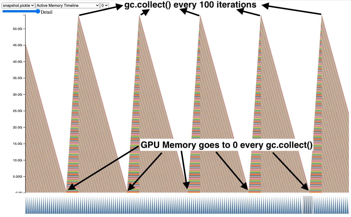
Although this works and fixes the CUDA OOM issue, calling gc.collect() too frequently can cause other issues including QPS regressions. Therefore we cannot simply increase the frequency of garbage collection on every training job. It’s best to just avoid creating reference cycles in the first place. More on this in section, Reference Cycle Detector.
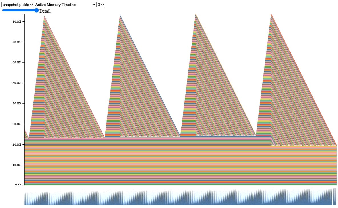
Sneaky Memory Leak in Callback
Real examples are more complicated, so let’s look at a more realistic example that has a similar behavior. In this snapshot, we can observe the same behavior of tensors being accumulated and freed during automatic garbage collection, until we hit a CUDA OOM.
Code Snippet behind this snapshot (full code sample in Appendix A):
class AwaitableTensor:
def __init__(self, tensor_size):
self._tensor_size = tensor_size
self._tensor = None
def wait(self):
self._tensor = torch.zeros(self._tensor_size, device="cuda:0")
return self._tensor
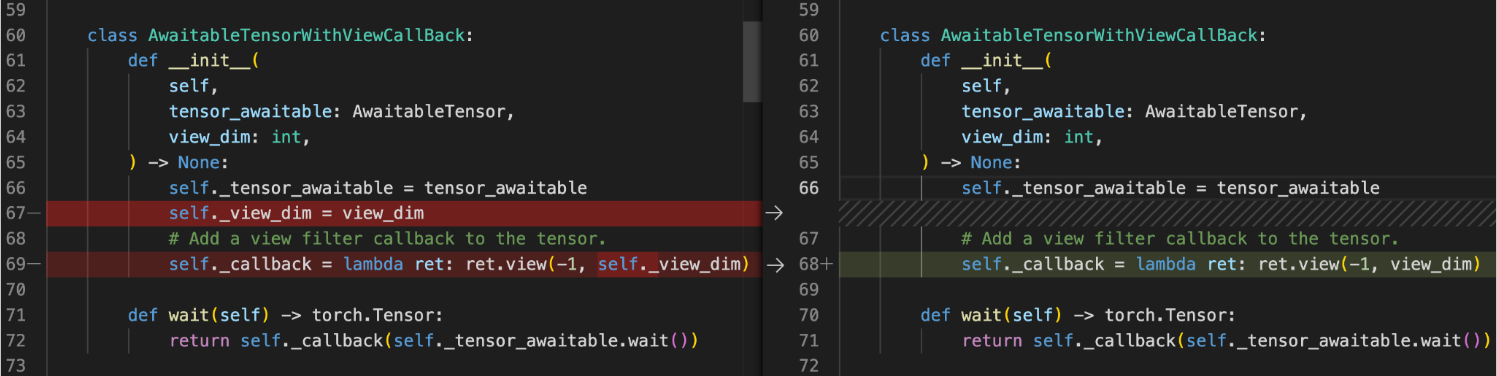
class AwaitableTensorWithViewCallback:
def __init__(self, tensor_awaitable, view_dim):
self._tensor_awaitable = tensor_awaitable
self._view_dim = view_dim
# Add a view filter callback to the tensor.
self._callback = lambda ret: ret.view(-1, self._view_dim)
def wait(self):
return self._callback(self._tensor_awaitable.wait())
async def awaitable_leak(
tensor_size=2**27, num_iter=100000,
):
for _ in range(num_iter):
A = AwaitableTensor(tensor_size)
AwaitableTensorWithViewCallBack(A, 4).wait()
In this code, we define two classes. The class AwaitableTensor will create a tensor when waited upon. Another class AwaitableTensorWithViewCallback will apply a view filter on the AwaitableTensor via callback lambda.
When running awaitable_leak, which creates tensor A (512 MB) and applies a view filter for 100,000 iterations, we expect that A should be reclaimed each time it goes out of scope because the reference count should reach 0. However, this will actually OOM!
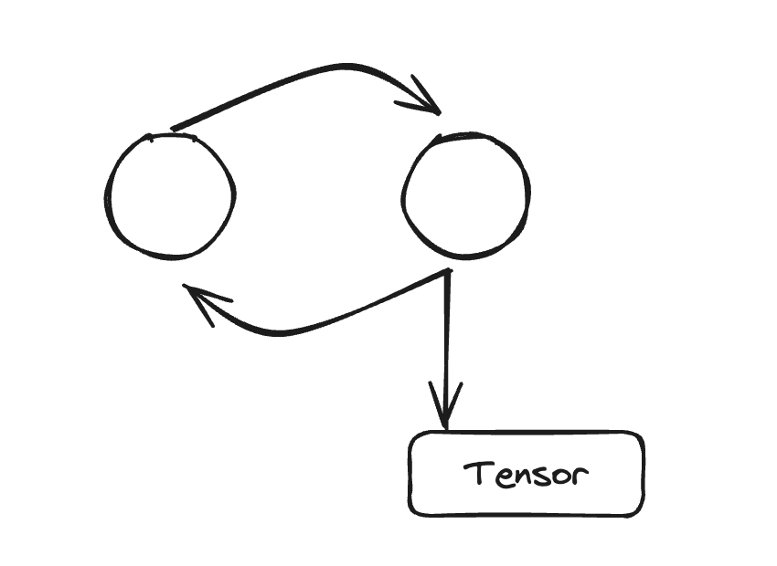
While we know there is a reference cycle here, it isn’t clear from the code where the cycle is created. To help with these situations, we have created a tool to locate and report these cycles.
Reference Cycle Detector
Introducing the Reference Cycle Detector, which helps us find reference cycles keeping GPU tensors alive. The API is fairly simple:
- During model initialization:
- Import:
from torch.utils.viz._cycles import warn_tensor_cycles - Start:
warn_tensor_cycles()
- Import:
The Reference Cycle Detector will issue warnings every time that the cycle collector runs and finds a CUDA tensor that gets freed. The warning provides an object graph showing how the reference cycle refers to the GPU tensor.
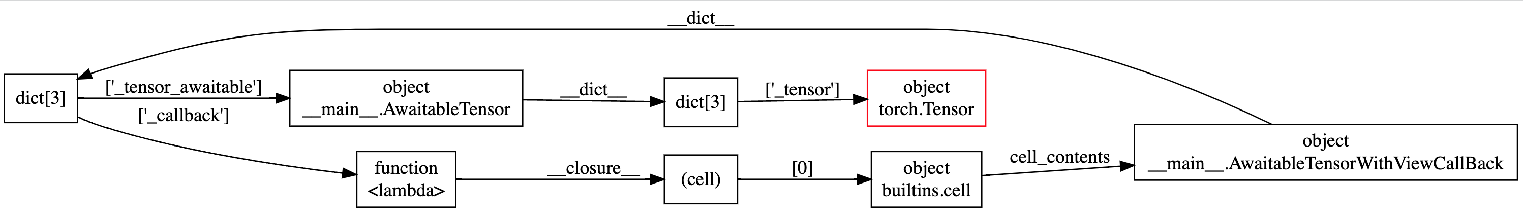
For instance in this object graph, we can easily observe that there is a circular dependency on the outer circle of the graph, and highlighted in red is the GPU tensor kept alive.
Most cycles are pretty easy to fix once they are discovered. For instance here we can remove the reference to self created by self._view_dim in the callback.
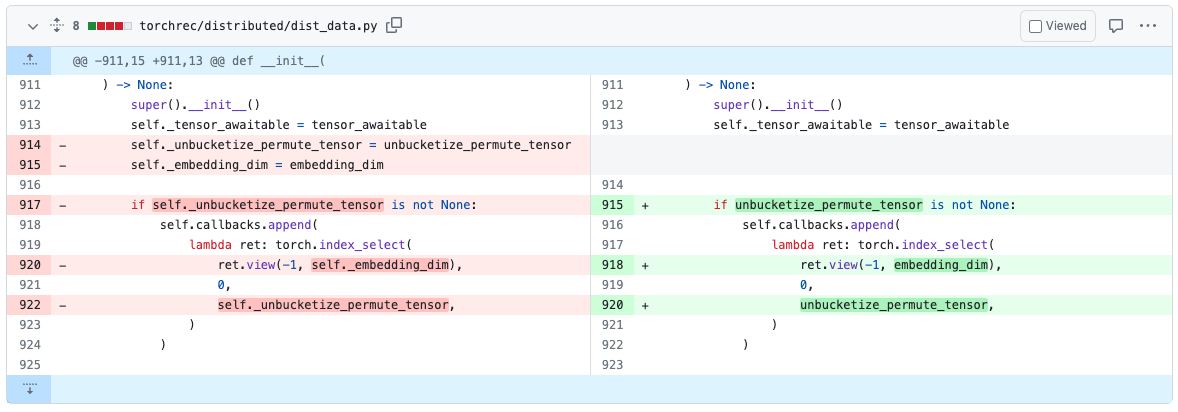
We’ve spent some time fixing cycles in existing models using these tools. For example in TorchRec, we’ve found and removed a reference cycle in PR#1226.
Once we’ve removed the reference cycles, the code will no longer issue a CUDA OOM nor show any memory leaks in their snapshots.
What are the other benefits of using the Reference Cycle Detector?
Removing these cycles will also directly lower the maximum GPU memory usage as well as make it less likely for memory to fragment because the allocator returns to the same state after each iteration.
Where can I find these tools?
We hope that the Reference Cycle Detector will greatly improve your ability to find and remove memory leaks caused by reference cycles. The Reference Cycle Detector is available in the v2.1 release of PyTorch as experimental features and More information about the Reference Cycle Detector can be found in the PyTorch Memory docs here.
Feedback
We look forward to hearing from you about any enhancements, bugs or memory stories that our tools helped to solve! As always, please feel free to open new issues on PyTorch’s Github page.
We are also open to contributions from the OSS community, feel free to tag Aaron Shi and Zachary DeVito in any Github PRs for reviews.
Acknowledgements
Really appreciate the content reviewers, Mark Saroufim, Gregory Chanan, and Adnan Aziz for reviewing this post and improving its readability.
Appendix
Appendix A – Code Sample
This code snippet was used to generate the plots and examples shown. Here are the arguments to reproduce the sections:
- Introduction:
python sample.py - Explicitly calling gc.collect():
python sample.py --gc_collect_interval=100 - Sneaky Memory Leak in Callback:
python sample.py --workload=awaitable - Ref Cycle Detector:
python sample.py --workload=awaitable --warn_tensor_cycles
sample.py:
# (c) Meta Platforms, Inc. and affiliates.
import argparse
import asyncio
import gc
import logging
import socket
from datetime import datetime, timedelta

import torch

logging.basicConfig(
   format="%(levelname)s:%(asctime)s %(message)s",
   level=logging.INFO,
   datefmt="%Y-%m-%d %H:%M:%S",
)
logger: logging.Logger = logging.getLogger(__name__)
logger.setLevel(level=logging.INFO)

TIME_FORMAT_STR: str = "%b_%d_%H_%M_%S"

# Keep a max of 100,000 alloc/free events in the recorded history
# leading up to the snapshot.
MAX_NUM_OF_MEM_EVENTS_PER_SNAPSHOT: int = 100000

def start_record_memory_history() -> None:
   if not torch.cuda.is_available():
       logger.info("CUDA unavailable. Not recording memory history")
       return

   logger.info("Starting snapshot record_memory_history")
   torch.cuda.memory._record_memory_history(
       max_entries=MAX_NUM_OF_MEM_EVENTS_PER_SNAPSHOT
   )

def stop_record_memory_history() -> None:
   if not torch.cuda.is_available():
       logger.info("CUDA unavailable. Not recording memory history")
       return

   logger.info("Stopping snapshot record_memory_history")
   torch.cuda.memory._record_memory_history(enabled=None)

def export_memory_snapshot() -> None:
   if not torch.cuda.is_available():
       logger.info("CUDA unavailable. Not exporting memory snapshot")
       return

   # Prefix for file names.
   host_name = socket.gethostname()
   timestamp = datetime.now().strftime(TIME_FORMAT_STR)
   file_prefix = f"{host_name}_{timestamp}"

   try:
       logger.info(f"Saving snapshot to local file: {file_prefix}.pickle")
       torch.cuda.memory._dump_snapshot(f"{file_prefix}.pickle")
   except Exception as e:
       logger.error(f"Failed to capture memory snapshot {e}")
       return

# This function will leak tensors due to the reference cycles.
def simple_leak(tensor_size, gc_interval=None, num_iter=30000, device="cuda:0"):
    class Node:
        def __init__(self, T):
            self.tensor = T
            self.link = None

    for i in range(num_iter):
        A = torch.zeros(tensor_size, device=device)
        B = torch.zeros(tensor_size, device=device)
        a, b = Node(A), Node(B)
        # A reference cycle will force refcounts to be non-zero, when
        # a and b go out of scope.
        a.link, b.link = b, a
        # Python will eventually gc a and b, but may OOM on the CUDA
        # device before that happens (since python runtime doesn't
        # know about CUDA memory usage).

        # Since implicit gc is not called frequently enough due to
        # generational gc, adding an explicit gc is necessary as Python
        # runtime does not know about CUDA memory pressure.
        # https://en.wikipedia.org/wiki/Tracing_garbage_collection#Generational_GC_(ephemeral_GC)
        if gc_interval and i % int(gc_interval) == 0:
            gc.collect()

async def awaitable_leak(
    tensor_size, gc_interval=None, num_iter=100000, device="cuda:0"
):
    class AwaitableTensor:
        def __init__(self, tensor_size, device) -> None:
            self._tensor_size = tensor_size
            self._device = device
            self._tensor = None

        def wait(self) -> torch.Tensor:
            self._tensor = torch.zeros(self._tensor_size, device=self._device)
            return self._tensor

    class AwaitableTensorWithViewCallBack:
        def __init__(
            self,
            tensor_awaitable: AwaitableTensor,
            view_dim: int,
        ) -> None:
            self._tensor_awaitable = tensor_awaitable
            self._view_dim = view_dim
            # Add a view filter callback to the tensor.
            self._callback = lambda ret: ret.view(-1, self._view_dim)

        def wait(self) -> torch.Tensor:
            return self._callback(self._tensor_awaitable.wait())

    for i in range(num_iter):
        # Create an awaitable tensor
        a_tensor = AwaitableTensor(tensor_size, device)

        # Apply a view filter callback on the awaitable tensor.
        AwaitableTensorWithViewCallBack(a_tensor, 4).wait()

        # a_tensor will go out of scope.

        if gc_interval and i % int(gc_interval) == 0:
            gc.collect()

if __name__ == "__main__":
    parser = argparse.ArgumentParser(description="A memory_leak binary instance")
    parser.add_argument(
        "--gc_collect_interval",
        default=None,
        help="Explicitly call GC every given interval. Default is off.",
    )
    parser.add_argument(
        "--workload",
        default="simple",
        help="Toggle which memory leak workload to run. Options are simple, awaitable.",
    )
    parser.add_argument(
        "--warn_tensor_cycles",
        action="store_true",
        default=False,
        help="Toggle whether to enable reference cycle detector.",
    )
    args = parser.parse_args()

    if args.warn_tensor_cycles:
        from tempfile import NamedTemporaryFile

        from torch.utils.viz._cycles import observe_tensor_cycles

        logger.info("Enabling warning for Python reference cycles for CUDA Tensors.")

        def write_and_log(html):
            with NamedTemporaryFile("w", suffix=".html", delete=False) as f:
                f.write(html)
                logger.warning(
                    "Reference cycle includes a CUDA Tensor see visualization of cycle %s",
                    f.name,
                )

        observe_tensor_cycles(write_and_log)
    else:
        # Start recording memory snapshot history
        start_record_memory_history()

    # Run the workload with a larger tensor size.
    # For smaller sizes, we will not CUDA OOM as gc will kick in often enough
    # to reclaim reference cycles before an OOM occurs.
    size = 2**26  # 256 MB
    try:
        if args.workload == "awaitable":
            size *= 2
            logger.info(f"Running tensor_size: {size*4/1024/1024} MB")
            asyncio.run(
                awaitable_leak(tensor_size=size, gc_interval=args.gc_collect_interval)
            )
        elif args.workload == "simple":
            logger.info(f"Running tensor_size: {size*4/1024/1024} MB")
            simple_leak(tensor_size=size, gc_interval=args.gc_collect_interval)
        else:
            raise Exception("Unknown workload.")
    except Exception:
        logger.exception(f"Failed to allocate {size*4/1024/1024} MB")

    # Create the memory snapshot file
    export_memory_snapshot()

    # Stop recording memory snapshot history
    stop_record_memory_history()

ISO 42001: A new foundational global standard to advance responsible AI

Artificial intelligence (AI) is one of the most transformational technologies of our generation and provides opportunities to be a force for good and drive economic growth. The growth of large language models (LLMs), with hundreds of billions of parameters, has unlocked new generative AI use cases to improve customer experiences, boost employee productivity, and so much more. At AWS, we remain committed to harnessing AI responsibly, working hand in hand with our customers to develop and use AI systems with safety, fairness, and security at the forefront.
The AI industry reached an important milestone this week with the publication of ISO 42001. In simple terms, ISO 42001 is an international management system standard that provides guidelines for managing AI systems within organizations. It establishes a framework for organizations to systematically address and control the risks related to the development and deployment of AI. ISO 42001 emphasizes a commitment to responsible AI practices, encouraging organizations to adopt controls specific to their AI systems, fostering global interoperability, and setting a foundation for the development and deployment of responsible AI.
Trust in AI is crucial and integrating standards such as ISO 42001, which promotes AI governance, is one way to help earn public trust by supporting a responsible use approach.
As part of a broad, international community of subject matter experts, AWS has actively collaborated in ISO 42001’s development since 2021 and started laying the foundation prior to the standard’s final publication.
International standards foster global cooperation in developing and implementing responsible AI solutions. Perhaps like no other technology before it, managing these challenges requires collaboration and a truly multidisciplinary effort across technology companies, policymakers, community groups, scientists, and others—and international standards play a valuable role.
International standards are an important tool to help organizations translate domestic regulatory requirements into compliance mechanisms, including engineering practices, that are largely globally interoperable. Effective standards help reduce confusion about what AI is and what responsible AI entails, and help focus the industry on the reduction of potential harms. AWS is working in a community of diverse international stakeholders to improve emerging AI standards on variety of topics, including risk management, data quality, bias, and transparency.
Conformance with the new ISO 42001 standard is one of the ways that organizations can demonstrate a commitment to excellence in responsibly developing and deploying AI systems and applications. We are continuing to pursue the adoption of ISO 42001, and look forward to working with customers to do the same.
We are committed to investing in the future of responsible AI, and helping to inform international standards in the interest of our customers and the communities in which we all live and operate.
About the authors
 Swami Sivasubramanian is Vice President of Data and Machine Learning at AWS. In this role, Swami oversees all AWS Database, Analytics, and AI & Machine Learning services. His team’s mission is to help organizations put their data to work with a complete, end-to-end data solution to store, access, analyze, and visualize, and predict.

AI Frontiers: A deep dive into deep learning with Ashley Llorens and Chris Bishop

Powerful large-scale AI models like GPT-4 are showing dramatic improvements in reasoning, problem-solving, and language capabilities. This marks a phase change for artificial intelligence—and a signal of accelerating progress to come.
In this Microsoft Research Podcast series, AI scientist and engineer Ashley Llorens hosts conversations with his collaborators and colleagues about what these models—and the models that will come next—mean for our approach to creating, understanding, and deploying AI, its applications in areas such as healthcare and education, and its potential to benefit humanity.
This episode features Technical Fellow Christopher Bishop (opens in new tab), who leads a global team of researchers and engineers working to help accelerate scientific discovery by merging machine learning and the natural sciences. Llorens and Bishop explore the state of deep learning; Bishop’s new textbook, Deep Learning: Foundations and Concepts (opens in new tab), his third and a writing collaboration with his son; and a potential future in which “super copilots” accessible via natural language and drawing on a variety of tools, like those that can simulate the fundamental equations of nature, are empowering scientists in their pursuit of breakthrough.

Learn more:
- Deep Learning: Foundations and Concepts (opens in new tab)
Textbook, 2023 - Pattern Recognition and Machine Learning
Textbook, 2006 - Neural Networks for Pattern Recognition
Textbook, 1995
Subscribe to the Microsoft Research Podcast:
Transcript
[MUSIC PLAYS]ASHLEY LLORENS: I’m Ashley Llorens with Microsoft Research. I’ve spent the last 20 years working in AI and machine learning, but I’ve never felt more excited to work in the field than right now. The latest foundation models and the systems we’re building around them are exhibiting surprising new abilities in reasoning, problem-solving, and translation across languages and domains. In this podcast series, I’m sharing conversations with fellow researchers about the latest developments in AI models, the work we’re doing to understand their capabilities and limitations, and ultimately how innovations like these can have the greatest benefit for humanity. Welcome to AI Frontiers.
Today, I’ll speak with Chris Bishop. Chris was educated as a physicist but has spent more than 25 years as a leader in the field of machine learning. Chris directs our AI4Science organization, which brings together experts in machine learning and across the natural sciences with the aim of revolutionizing scientific discovery.
[MUSIC FADES]
So, Chris, you have recently published a new textbook on deep learning, maybe the new definitive textbook on deep learning. Time will tell. So, of course, I want to get into that. But first, I’d like to dive right into a few philosophical questions. In the preface of the book, you make reference to the massive scale of state-of-the-art language models, generative models comprising on the order of a trillion learnable parameters. How well do you think we understand what a system at that scale is actually learning?
CHRIS BISHOP: That’s a super interesting question, Ashley. So in one sense, of course, we understand the systems extremely well because we designed them; we built them. But what’s very interesting about machine learning technology compared to most other technologies is that the, the functionality in large part is learned, is learned from data. And what we discover in particular with these very large language models is, kind of, emergent behavior. As we go up at each factor of 10 in scale, we see qualitatively new properties and capabilities emerging. And that’s super interesting. That, that was called the scaling hypothesis. And it’s proven to be remarkably successful.
LLORENS: Your new book lays out foundations in statistics and probability theory for modern machine learning. Central to those foundations is the concept of probability distributions, in particular learning distributions in the service of helping a machine perform a useful task. For example, if the task is object recognition, we may seek to learn the distribution of pixels you’d expect to see in images corresponding to objects of interest, like a teddy bear or a racecar. On smaller scales, we can at least conceive of the distributions that machines are learning. What does it mean to learn a distribution at the scale of a trillion learnable parameters?
BISHOP: Right. That’s really interesting. So, so first of all, the fundamentals are very solid. The fact that we have this, this, sort of, foundational rock of probability theory on which everything is built is extremely powerful. But then these emergent properties that we talked about are the result of extremely complex statistics. What’s really interesting about these neural networks, let’s say, in comparison with the human brain is that we can perform perfect diagnostics on them. We can understand exactly what each neuron is doing at each moment of time. And, and so we can almost treat the system in a, in a, sort of, somewhat experimental way. We can, we can probe the system. You can apply different inputs and see how different units respond. You can play games like looking at a unit that responds to a particular input and then perhaps amplifying the, amplifying that response, adjusting the input to make that response stronger, seeing what effect it has, and so on. So there’s an aspect of machine learning these days that’s somewhat like experimental neurobiology, except with the big advantage that we have sort of perfect diagnostics.
LLORENS: Another concept that is key in machine learning is generalization. In more specialized systems, often smaller systems, we can actually conceive of what we might mean by generalizing. In the object recognition example I used earlier, we may want to train an AI model capable of recognizing any arbitrary image of a teddy bear. Because this is a specialized task, it is easy to grasp what we mean by generalization. But what does generalization mean in our current era of large-scale AI models and systems?
BISHOP: Right. Well, generalization is a fundamental property, of course. If we couldn’t generalize, there’d be no point in building these systems. And again, these, these foundational principles apply equally at a very large scale as they do at a, at a smaller scale. But the concept of generalization really has to do with modeling the distribution from which the data is generated. So if you think about a large language model, it’s trained by predicting the next word or predicting the next token. But really what we’re doing is, is creating a task for the model that forces it to learn the underlying distribution. Now, that distribution may be extremely complex, let’s say, in the case of natural language. It can convey a tremendous amount of meaning. So, really, the system is forced to … in order to get the best possible performance, in order to make the best prediction for the next word, if you like, it’s forced to effectively understand the meaning of the content of the data. In the case of language, the meaning of effectively what’s being said. And so from a mathematical point of view, there’s a very close relationship between learning this probability distribution and the problem of data compression, because it turns out if you want to compress data in a lossless way, the optimal way to do that is to learn the distribution that generates the data. So that’s, that’s … we show that in the book, in fact. And so, and the best way to … let’s take the example of images, for instance. If you’ve got a very, very large number of natural images and you had to compress them, the most efficient way to compress them would be to understand the mechanisms by which the images come about. There are objects. You could, you could pick a car or a bicycle or a house. There’s lighting from different angles, shadows, reflections, and so on. And learning about those mechanisms—understanding those mechanisms—will give you the best possible compression, but it’ll also give you the best possible generalization.
LLORENS: Let’s talk briefly about one last fundamental concept—inductive bias. Of course, as you mentioned, AI models are learned from data and experience, and my question for you is, to what extent do the neural architectures underlying those models represent an inductive bias that shapes the learning?
BISHOP: This is a really interesting question, as well, and it sort of reflects the journey that neural nets have been on in the last, you know, 30–35 years since we first started using gradient-based methods to train them. So, so the idea of inductive bias is that, actually, you can only learn from data in the presence of assumptions. There’s, actually, a theorem called the “no free lunch” theorem, which proves this mathematically. And so, to be able to generalize, you have to have data and some sort of assumption, some set of assumptions. Now, if you go back, you know, 30 years, 35 years, when I first got excited about neural nets, we had very simple one– and two–layered neural nets. We had to put a lot of assumptions in. We’d have to code a lot of human expert knowledge into feature extraction, and then the neural net would do a little bit of, the last little bit of work of just mapping that into a, sort of, a linear representation and then, then learning a classifier or whatever it was. And then over the years as we’ve learned to train bigger and richer neural nets, we can allow the data to have more influence and then we can back off a little bit on some of that prior knowledge. And today, when we have models like large-scale transformers with a trillion parameters learned on vast datasets, we’re letting the data do a lot of the heavy lifting. But there always has to be some kind of assumption. So in the case of transformers, there are inductive biases related to the idea of attention. So that’s a, that’s a specific structure that we bake into the transformer, and that turns out to be very, very successful. But there’s always inductive bias somewhere.
LLORENS: Yeah, and I guess with these new, you know, generative pretrained models, there’s also some inductive bias you’re imposing in the inferencing stage, just with your, with the way you prompt the system.
BISHOP: And, again, this is really interesting. The whole field of deep learning has become incredibly rich in terms of pretraining, transfer learning, the idea of prompting, zero-shot learning. The field has exploded really in the last 10 years—the last five years—not just in terms of the number of people and the scale of investment, number of startups, and so on, but the sort of the richness of ideas and, and, and techniques like, like order differentiation, for example, that mean we don’t have to code up all the gradient optimization steps. It allows us to explore a tremendous variety of different architectures very easily, very readily. So it’s become just an amazingly exciting field in the last decade.
LLORENS: And I guess we’ve, sort of, intellectually pondered here in the first few minutes the current state of the field. But what was it like for you when you first used, you know, a state-of-the-art foundation model? What was that moment like for you?
BISHOP: Oh, I could remember it clearly. I was very fortunate because I was given, as you were, I think, a very early access to GPT-4, when it was still very secret. And I, I’ve described it as being like the, kind of, the five stages of grief. It’s a, sort of, an emotional experience actually. Like first, for me, it was, like, a, sort of, first encounter with a primitive intelligence compared to human intelligence, but nevertheless, it was … it felt like this is the first time I’ve ever engaged with an intelligence that was sort of human-like and had those first sparks of, of human-level intelligence. And I found myself going through these various stages of, first of all, thinking, no, this is, sort of, a parlor trick. This isn’t real. And then, and then it would do something or say something that would be really quite shocking and profound in terms of its … clearly it was understanding aspects of what was being discussed. And I’d had several rounds of that. And then, then the next, I think, was that real? Did I, did I imagine that? And go back and try again and, no, there really is something here. So, so clearly, we have quite a way to go before we have systems that really match the incredible capabilities of the human brain. But nevertheless, I felt that, you know, after 35 years in the field, here I was encountering the first, the first sparks, the first hints, of real machine intelligence.
LLORENS: Now let’s get into your book. I believe this is your third textbook. You contributed a text called Neural Networks for Pattern Recognition in ’95 and a second book called Pattern Recognition and Machine Learning in 2006, the latter still being on my own bookshelf. So I think I can hazard a guess here, but what inspired you to start writing this third text?
BISHOP: Well, really, it began with … actually, the story really begins with the COVID pandemic and lockdown. It was 2020. The 2006 Pattern Recognition and Machine Learning book had been very successful, widely adopted, still very widely used even though it predates the, the deep learning revolution, which of course one of the most exciting things to happen in the field of machine learning. And so it’s long been on my list of things to do, to update the book, to bring it up to date, to include deep learning. And when the, when the pandemic lockdown arose, 2020, I found myself sort of imprisoned, effectively, at home with my family, a very, very happy prison. But I needed a project. And I thought this would be a good time to start to update the book. And my son, Hugh, had just finished his degree in computer science at Durham and was embarking on a master’s degree at Cambridge in machine learning, and we decided to do this as a joint project during, during the lockdown. And we’re having a tremendous amount of fun together. We quickly realized, though, that the field of deep learning is so, so rich and obviously so important these days that what we really needed was a new book rather than merely, you know, a few extra chapters or an update to a previous book. And so we worked on that pretty hard for nearly a couple of years or so. And then, and then the story took another twist because Hugh got a job at Wayve Technologies in London building deep learning systems for autonomous vehicles. And I started a new team in Microsoft called AI4Science. We both found ourselves extremely busy, and the whole project, kind of, got put on the back burner. And then along came GPT and ChatGPT, and that, sort of, exploded into the world’s consciousness. And we realized that if ever there was a time to finish off a textbook on deep learning, this was the moment. And so the last year has really been absolutely flat out getting this ready, in fact, ready in time for launch at NeurIPS this year.
LLORENS: Yeah, you know, it’s not every day you get to do something like write a textbook with your son. What was that experience like for you?
BISHOP: It was absolutely fabulous. And, and I hope it was good fun for Hugh, as well. You know, one of the nice things was that it was a, kind of, a pure collaboration. There was no divergence of agendas or any sense of competition. It was just pure collaboration. The two of us working together to try to understand things, try to work out what’s the best way to explain this, and if we couldn’t figure something out, we’d go to the whiteboard together and sketch out some maths and try to understand it together. And it was just tremendous fun. Just a real, a real pleasure, a real honor, I would say.
LLORENS: One of the motivations that you articulate in the preface of your book is to make the field of deep learning more accessible for newcomers to the field. Which makes me wonder what your sense is of how accessible machine learning actually is today compared to how it was, say, 10 years ago. On the one hand, I personally think that the underlying concepts around transformers and foundation models are actually easier to grasp than the concepts from previous eras of machine learning. Today, we also see a proliferation of helpful packages and toolkits that people can pick up and use. And on the other hand, we’ve seen an explosion in terms of the scale of compute necessary to do research at the frontiers. So net, what’s your concept of how accessible machine learning is today?
BISHOP: I think you’ve hit on some good points there. I would say the field of machine learning has really been through these three eras. The first was the focus on neural networks. The second was when, sort of, neural networks went into the back burner. As you, you hinted there, there was a proliferation of different ideas—Gaussian processes, graphical models, kernel machines, support vector machines, and so on—and the field became very broad. There are many different concepts to, to learn. Now, in a sense, it’s narrowed. The focus really is on deep neural networks. But within that field, there has been an explosion of different architectures and different … and not only in terms of the number of architectures. Just the sheer number of papers published has, has literally exploded. And, and so it can be very daunting, very intimidating, I think, especially for somebody coming into the field afresh. And so really the value proposition of this book is distill out the, you know, 20 or so foundational ideas and concepts that you really need to understand in order to understand the field. And the hope is that if you’ve really understood the content of the book, you’d be in pretty good shape to pretty much read any, any paper that’s published. In terms of actually using the technology in practice, yes, on the one hand, we have these wonderful packages and, especially with all the differentiation that I mentioned before, is really quite revolutionary. And now you can, you can put things together very, very quickly, a lot of open-source code that you can quickly bolt together and assemble lots of different, lots of different things, try things out very easily. It’s true, though, that if you want to operate at the very cutting edge of large-scale machine learning, that does require resources on a very large scale. So that’s obviously less accessible. But if your goal is to understand the field of machine learning, then, then I hope the book will serve a good purpose there. And in one sense, the fact that the packages are so accessible and so easy to use really hides some of the inner workings, I would say, of these, of these systems. And so I think in a way, it’s almost too easy just to train up a neural network on some data without really understanding what’s going on. So, so the book is really about, if you like, the minimum set of things that you need to know about in order to understand the field, not just to, sort of, turn the crank on it on a package but really understand what’s going on inside.
LLORENS: One of the things I think you did not set out to do, as you just mentioned, is to create an exhaustive survey of the most recent advancements, which might have been possible, you know, a decade or so ago. How do you personally keep up with the blistering pace of research these days?
BISHOP: Ah, yes, it’s a, it’s a challenge, of course. So, so my focus these days is on AI4Science, AI for natural science. But that’s also becoming a very large field. But, you know, one of the, one of the wonderful things about being at Microsoft Research is just having fantastic colleagues with tremendous expertise. And so, a lot of what I learn is from, is from colleagues. And we’re often swapping notes on, you know, you should take a look at this paper, did you hear about this idea, and so on, and brainstorming things together. So a lot of it is, you know, just taking time each day to read papers. That’s important. But also, just conversations with, with colleagues.
LLORENS: OK, you mentioned AI4Science. I do want to get into that. I know it’s an area that you’re passionate about and one that’s become a focus for your career in this moment. And, you know, I think of our work in AI4Science as creating foundation models that are fluent not in human language but in the language of nature. And earlier in this conversation, we talked about distribution. So I want to, kind of, bring you back there. Do you think we can really model all of nature as one wildly complex statistical distribution?
BISHOP: [LAUGHS] Well, that’s, that’s really interesting. I do think I could imagine a future, maybe not too many years down the road, where scientists will engage with the tools of scientific discovery through something like a natural language model. That model will also have understanding of concepts around the structures of molecules and the nature of data, will read scientific literature, and so on, and be able to assemble these ideas together. But it may need to draw upon other kinds of tools. So whether everything will be integrated into one, one overarching tool is less clear to me because there are some aspects of scientific discovery that are being, truly being revolutionized right now by deep learning. For example, our ability to simulate the fundamental equations of nature is being transformed through deep learning, and the nature of that transformation, on the one hand, it leverages, might leverage architectures like diffusion models and large language, large language models, large transformers, and the ability to train on large GPU clusters. But the fundamental goals there are to solve differential equations at a very large scale. And so the kinds of techniques we use there are a little bit different from the ones we’d use in processing natural language, for example. So you could imagine, maybe not too many years in the future, where a scientist will have a, kind of, “super copilot” that they can interact with directly in natural language. And that copilot or system of copilots can itself draw upon various tools. They may be tools that simulate Schrödinger equation, solves Schrödinger equation, to predict the properties of molecules. It might call upon large-scale deep learning emulators that can do a similar thing to the simulators but very, very much more efficiently. It might even call upon automated labs, wet labs, that can run experiments and gather data and can help the scientist marshal these resources and make optimal decisions as they go through that iterative scientific discovery process, whether inventing a new battery, electrolyte, or whether discovering a new drug, for example.
LLORENS: We talked earlier about the “no free lunch” theorem and the concept of inductive bias. What does that look like here in training science foundation models?
BISHOP: Well, it’s really interesting, and maybe I’m a little biased because my background is in physics. I did a PhD in quantum field theory many decades ago. For me, one of the reasons that this is such an exciting field is that, you know, my own career has come full circle. I now get to combine machine learning with physics and chemistry and biology. I think the inductive bias here is, is particularly interesting. If you think about large language models, we don’t have very many, sort of, fundamental rules of language. I mean, the rules of linguistics are really human observations about the structure of language. But neural nets are very good at extracting that, that kind of structure from data. Whereas when we look at physics, we have laws which we believe hold very accurately. For example, conservation of energy or rotational invariance. The energy of a molecule in a vacuum doesn’t depend on its rotation in space, for example. And that kind of inductive bias is very rigorous. We believe that it holds exactly. And so there is … and also, very often, we want to train on data that’s obtained from simulators. So the training data itself is obtained by solving some of those fundamental equations, and that process itself is computationally expensive. So the data can often be in relatively limited supply. So you’re in a regime that’s a little bit different from the large language models. It’s a little bit more like, in a way, machine learning was, you know, 10 to 20 years ago, as you were talking about, where data, data is limited. But now we have these powerful and strong inductive biases, and so there’s, it’s a very rich field of research for how to build in those inductive biases into the machine learning models but in a way that retains computational efficiency. So I personally, actually, find this one of the most exciting frontiers not only of the natural sciences but also of machine learning.
LLORENS: Yeah, you know, physics and our understanding of the natural world has come so far, you know, over the last, you know, centuries and decades. And yet our understanding of physics is evolving. It’s an evolving science. And so maybe I’ll ask you somewhat provocatively if baking our current understanding of physics into these models as inductive biases is limiting in some way, perhaps limiting their ability to learn new physics?
BISHOP: It’s a great question. I think for the kinds of things that we’re particularly interested in, in Microsoft Research, in the AI4Science team, we’re very interested in things that have real-world applicability, things to do with drug discovery, materials design. And there, first of all, we do have a very good understanding of the fundamental equations, essentially Schrödinger equation and fundamental equations of physics, and those inductive biases such as energy conservation. We really do believe they hold very accurately in the domains that we’re interested in. However, there’s a lot of scientific knowledge that is, that represents approximations to that, because you can only really solve these equations exactly for very small systems. And as you start to get to larger, more complex systems, there are, as it were, laws of physics that aren’t, aren’t quite as rigorous, that are somewhat more empirically derived, where there perhaps is scope for learning new kinds of physics. And, certainly, as you get to larger systems, you get, you get emergent properties. So, so conservation of energy doesn’t get violated, but nevertheless, you can have a very interesting new emergent physics. And so it’s, from the point of view of scientific discovery, I think the field is absolutely wide open. If you look at solid-state physics, for example, and device physics, there’s a tremendous amount of exciting new research to be done over the coming decades.
LLORENS: Yeah, you alluded to this. I think maybe it’s worth just double clicking on for a moment because there is this idea of compositionality and emergent properties as you scale up, and I wonder if you could just elaborate on that a little bit.
BISHOP: Yeah, that’s a good, that’s a good, sort of, picture to have this, sort of, hierarchy of different levels in the way they interact with each other. And at the very deepest level, the level of electrons, you might even more or less directly solve Schrödinger equation or do some very good approximation to that. That quickly becomes infeasible. And as you go up this hierarchy of, effectively, length scales, you have to make more and more approximations in order to be computationally efficient or computationally even practical. But in a sense, the previous levels of the hierarchy can provide you with training data and with validation verification of what you’re doing at the next level. And so the interplay between these different hierarchies is also very, very, very interesting. So at the level of electrons, they govern forces between atoms, which governs the dynamics of atoms. But once you look at larger molecules, you perhaps can’t simulate the behavior of every electron. You have to make some approximations. And then for larger molecules still, you can’t even track the behavior of every atom. You need some sort of coarse graining and so on. And so you have this, this hierarchy of different length scales. But every single one of those length scales is being transformed by deep learning, by our ability to learn from simulations, learn from those fundamental equations, in some cases, learn also from experimental data and build emulators, effectively, systems that can simulate that particular length scale and the physical and biological properties but do so in a way that’s computationally very efficient. So every layer of this hierarchy is currently being transformed, which is just amazingly exciting.
LLORENS: You alluded to some of the application domains that stand to get disrupted by advancements in AI4Science. What are a couple of the applications that you’re most excited about?
BISHOP: There are so many, it would be impossible to list them. But let me give you a couple of domains. I mean, the first one is, is healthcare and the ability to design new molecules, whether it’s small-molecule drugs or more protein-based therapies. That, that whole field is rapidly shifting to a much more computational domain, and that should accelerate our ability to develop new therapies, new drugs. The other class of domains has more to do with materials, and there are a lot of … the applications that we’re interested in relate to sustainability, things to do with capturing CO2 from the atmosphere, creating, let’s say, electricity from hydrogen, creating hydrogen from electricity. We need to do things both ways round. Just storing heat as a form of energy storage. Many, many applications relating to sustainability to do with, to do with protecting our water supply, to do with providing green energy, to do with storing and transporting energy. Many, many applications.
LLORENS: And at the core of all those advancements is deep learning as we’ve kind of started. And so maybe as we, as we close, we can, kind of, come back to your book on deep learning. I don’t have the physical book yet, but there’s a spot on my shelf next to your last book that’s waiting for it. But as we close here, maybe you can tell folks where to look for or how to get a copy of your new book.
BISHOP: Oh, sure. It’s dead easy. You go to bishopbook.com, and from there, you’ll see how to order a hardback copy if that’s what you’d like, or there’s a PDF based e-book version. There’ll be a Kindle version, I believe. But there’s also a free-to-use online version on bishopbook.com, and it’s available there. It’s, sort of, PDF style and fully hyperlinked, free to use, and I hope people will read it, and enjoy it, and learn from it.
LLORENS: Thanks for a fascinating discussion, Chris.
BISHOP: Thanks, Ashley.
The post AI Frontiers: A deep dive into deep learning with Ashley Llorens and Chris Bishop appeared first on Microsoft Research.
Accelerating time-to-insight with MongoDB time series collections and Amazon SageMaker Canvas
This is a guest post co-written with Babu Srinivasan from MongoDB.
As industries evolve in today’s fast-paced business landscape, the inability to have real-time forecasts poses significant challenges for industries heavily reliant on accurate and timely insights. The absence of real-time forecasts in various industries presents pressing business challenges that can significantly impact decision-making and operational efficiency. Without real-time insights, businesses struggle to adapt to dynamic market conditions, accurately anticipate customer demand, optimize inventory levels, and make proactive strategic decisions. Industries such as Finance, Retail, Supply Chain Management, and Logistics face the risk of missed opportunities, increased costs, inefficient resource allocation, and the inability to meet customer expectations. By exploring these challenges, organizations can recognize the importance of real-time forecasting and explore innovative solutions to overcome these hurdles, enabling them to stay competitive, make informed decisions, and thrive in today’s fast-paced business environment.
By harnessing the transformative potential of MongoDB’s native time series data capabilities and integrating it with the power of Amazon SageMaker Canvas, organizations can overcome these challenges and unlock new levels of agility. MongoDB’s robust time series data management allows for the storage and retrieval of large volumes of time-series data in real-time, while advanced machine learning algorithms and predictive capabilities provide accurate and dynamic forecasting models with SageMaker Canvas.
In this post, we will explore the potential of using MongoDB’s time series data and SageMaker Canvas as a comprehensive solution.
MongoDB Atlas
MongoDB Atlas is a fully managed developer data platform that simplifies the deployment and scaling of MongoDB databases in the cloud. It is a document based storage that provides a fully managed database, with built-in full-text and vector Search, support for Geospatial queries, Charts and native support for efficient time series storage and querying capabilities. MongoDB Atlas offers automatic sharding, horizontal scalability, and flexible indexing for high-volume data ingestion. Among all, the native time series capabilities is a standout feature, making it ideal for a managing high volume of time-series data, such as business critical application data, telemetry, server logs and more. With efficient querying, aggregation, and analytics, businesses can extract valuable insights from time-stamped data. By using these capabilities, businesses can efficiently store, manage, and analyze time-series data, enabling data-driven decisions and gaining a competitive edge.
Amazon SageMaker Canvas
Amazon SageMaker Canvas is a visual machine learning (ML) service that enables business analysts and data scientists to build and deploy custom ML models without requiring any ML experience or having to write a single line of code. SageMaker Canvas supports a number of use cases, including time-series forecasting, which empowers businesses to forecast future demand, sales, resource requirements, and other time-series data accurately. The service uses deep learning techniques to handle complex data patterns and enables businesses to generate accurate forecasts even with minimal historical data. By using Amazon SageMaker Canvas capabilities, businesses can make informed decisions, optimize inventory levels, improve operational efficiency, and enhance customer satisfaction.
The SageMaker Canvas UI lets you seamlessly integrate data sources from the cloud or on-premises, merge datasets effortlessly, train precise models, and make predictions with emerging data—all without coding. If you need an automated workflow or direct ML model integration into apps, Canvas forecasting functions are accessible through APIs.
Solution overview
Users persist their transactional time series data in MongoDB Atlas. Through Atlas Data Federation, data is extracted into Amazon S3 bucket. Amazon SageMaker Canvas access the data to build models and create forecasts. The results of the forecasting are stored in an S3 bucket. Using the MongoDB Data Federation services, the forecasts are presented visually through MongoDB Charts.
The following diagram outlines the proposed solution architecture.

Prerequisites
For this solution we use MongoDB Atlas to store time series data, Amazon SageMaker Canvas to train a model and produce forecasts, and Amazon S3 to store data extracted from MongoDB Atlas.
Make sure you have the following prerequisites:
Configure MongoDB Atlas cluster
Create a free MongoDB Atlas cluster by following the instructions in Create a Cluster. Setup the Database access and Network access.
Populate a time series collection in MongoDB Atlas
For the purposes of this demonstration, you can use a sample data set from from Kaggle and upload the same to MongoDB Atlas with the MongoDB tools , preferably MongoDB Compass.
The following code shows a sample data set for a time series collection:
{
"store": "1 1",
"timestamp": { "2010-02-05T00:00:00.000Z"},
"temperature": "42.31",
"target_value": 2.572,
"IsHoliday": false
}
The following screenshot shows the sample time series data in MongoDB Atlas:

Create an S3 Bucket
Create an S3 bucket in AWS , where the time series data need to be stored and analyzed. Note we have two folders. sales-train-data is used to store data extracted from MongoDB Atlas, while sales-forecast-output contains predictions from Canvas.

Create the Data Federation
Setup the Data Federation in Atlas and register the S3 bucket created previously as part of the data source. Notice the three different database/collections are created in the data federation for Atlas cluster, S3 bucket for MongoDB Atlas data and S3 bucket to store the Canvas results.
The following screenshots shows the setup of the data federation.

Setup the Atlas application service
Create the MongoDB Application Services to deploy the functions to transfer the data from MongoDB Atlas cluster to S3 bucket using the $out aggregation.

Verify the Datasource Configuration
The Application services create a new Altas Service Name that needs to be referred as the data services in the following function. Verify that the Atlas Service Name is created and note it for future reference.

Create the function
Setup the Atlas Application services to create the trigger and functions. The triggers need to be scheduled to write the data to S3 at a period frequency based on the business need for training the models.
The following script shows the function to write to the S3 bucket:
exports = function () {

   const service = context.services.get("");
   const db = service.db("")
   const events = db.collection("");

   const pipeline = [
    {
            "$out": {
               "s3": {
                  "bucket": "<S3_bucket_name>",
                  "region": "<AWS_Region>",
                   "filename": {$concat: ["<S3path>/<filename>_",{"$toString":  new Date(Date.now())}]},
                  "format": {
                        "name": "json",
                        "maxFileSize": "10GB"
                  }
               }
            }
      }
   ];

   return events.aggregate(pipeline);
};
Sample function
The function can be run through the Run tab and the errors can be debugged using the log features in the Application Services. In addition, the errors can be debugged using the Logs menu in the left pane.
The following screenshot shows the execution of the function along with the output:

Create dataset in Amazon SageMaker Canvas
The following steps assume that you have created a SageMaker domain and user profile. If you have not already done so, make sure that you configure the SageMaker domain and user profile. In the user profile, update your S3 bucket to be custom and supply your bucket name.

When complete, navigate to SageMaker Canvas, select your domain and profile, and select Canvas.

Create a dataset supplying the data source.

Select the dataset source as S3

Select the data location from the S3 bucket and select Create dataset.

Review the schema and click Create dataset

Upon successful import, the dataset will appear in the list as shown in the following screenshot.

Train the model
Next, we will use Canvas to set up to train the model. Select the dataset and click Create.

Create a model name, select Predictive analysis, and select Create.

Select target column

Next, click Configure time series model and select item_id as the Item ID column.

Select tm for the time stamp column

To specify the amount of time that you want to forecast, choose 8 weeks.

Now you are ready to preview the model or launch the build process.

After you preview the model or launch the build, your model will be created and can take up to four hours. You can leave the screen and return to see the model training status.

When the model is ready, select the model and click on the latest version

Review the model metrics and column impact and if you are satisfied with the model performance, click Predict.

Next, choose Batch prediction, and click Select dataset.

Select your dataset, and click Choose dataset.

Next, click Start Predictions.

Observe a job created or observe the job progress in SageMaker under Inference, Batch transform jobs.


When the job completes, select the job, and note the S3 path where Canvas stored the predictions.

Visualize forecast data in Atlas Charts
To visualize forecast data, create the MongoDB Atlas charts based on the Federated data (amazon-forecast-data) for P10, P50, and P90 forecasts as shown in the following chart.

Clean up
- Delete the MongoDB Atlas cluster
- Delete Atlas Data Federation Configuration
- Delete Atlas Application Service App
- Delete the S3 Bucket
- Delete Amazon SageMaker Canvas dataset and models
- Delete the Atlas Charts
- Log out of Amazon SageMaker Canvas
Conclusion
In this post we extracted time series data from MongoDB time series collection. This is a special collection optimized for storage and querying speed of time series data. We used Amazon SageMaker Canvas to train models and generate predictions and we visualized the predictions in Atlas Charts.
For more information, refer to the following resources.
- Try out MongoDB Atlas
- Try out MongoDB Atlas Time Series
- Try out Amazon SageMaker Canvas
- Try out MongoDB Charts
About the authors
 Igor Alekseev is a Senior Partner Solution Architect at AWS in Data and Analytics domain. In his role Igor is working with strategic partners helping them build complex, AWS-optimized architectures. Prior joining AWS, as a Data/Solution Architect he implemented many projects in Big Data domain, including several data lakes in Hadoop ecosystem. As a Data Engineer he was involved in applying AI/ML to fraud detection and office automation.
 Babu Srinivasan is a Senior Partner Solutions Architect at MongoDB. In his current role, he is working with AWS to build the technical integrations and reference architectures for the AWS and MongoDB solutions. He has more than two decades of experience in Database and Cloud technologies . He is passionate about providing technical solutions to customers working with multiple Global System Integrators(GSIs) across multiple geographies.
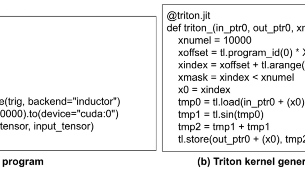
Training Production AI Models with PyTorch 2.0
1. Introduction
PyTorch 2.0 (abbreviated as PT2) can significantly improve the training and inference performance of an AI model using a compiler called_ torch.compile_ while being 100% backward compatible with PyTorch 1.x. There have been reports on how PT2 improves the performance of common benchmarks (e.g., huggingface’s diffusers). In this blog, we discuss our experiences in applying PT2 to production _AI models _at Meta.
2. Background
2.1 Why is automatic performance optimization important for production?
Performance is particularly important for production—e.g, even a 5% reduction in the training time of a heavily used model can translate to substantial savings in GPU cost and data-center power. Another important metric is development efficiency, which measures how many engineer-months are required to bring a model to production. Typically, a significant part of this bring-up effort is spent on manual _performance tuning such as rewriting GPU kernels to improve the training speed. By providing _automatic _performance optimization, PT2 can improve _both cost and development efficiency.
2.2 How PT2 improves performance
As a compiler, PT2 can view_ multiple_ operations in the training graph captured from a model (unlike in PT1.x, where only one operation is executed at a time). Consequently, PT2 can exploit a number of performance optimization opportunities, including:
- Fusing multiple operations into a single GPU kernel:
- A typical type of performance overhead in running a GPU program is the CPU overhead of launching small GPU kernels. By fusing multiple operations into a single GPU kernel, PT2 can significantly reduce the kernel-launching overhead on the CPU. For instance, consider the PyTorch program in Figure 1(a). When it is executed on GPU with PT1, it has three GPU kernels (two for the two sin() ops and one for the addition op). With PT2, there is only one kernel generated, which fuses all three ops.
- After fusing some operations, certain operations in the graph may become dead and hence can be optimized away. This can save both compute and memory bandwidth on the GPU. For instance, in Figure 1(b), one of the duplicated sin() ops can be optimized away.
- In addition, fusion can also reduce GPU device memory reads/writes (by composing pointwise kernels) and help improve hardware utilization.
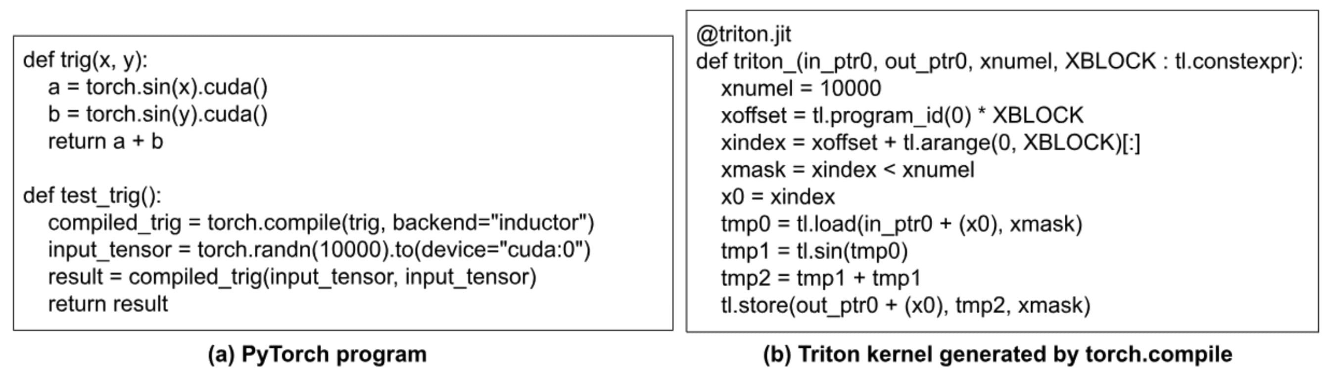
Fig. 1: How PT2 improves performance with fusion and dead-code elimination.
- Reducing the type conversion overhead for using lower-precision data types:
- PyTorch 1.x supports Automatic Mixed Precision (AMP). While AMP can reduce the compute time of an op, it introduces type conversion overhead before and after the op. PT2 can increase AMP performance by optimizing away unnecessary type conversion code, significantly reducing its overhead. As an example, Figure 2(a) converts three 32-bit input tensors (a32, b32, c32) to bf16 before doing the matrix multiplications. Nevertheless, in this example, a32 and c32 are actually the same tensor (a_float32). So, there is no need to convert a_float32 twice, as shown in the code generated by torch.compile in Figure 2(b). Note that while both this example and the previous one optimize away redundant computations, they are different in the sense that the type conversion code in this example is implicit via torch.autocast, unlike in the previous example where the torch.sin(x).cuda() is explicit in user code.
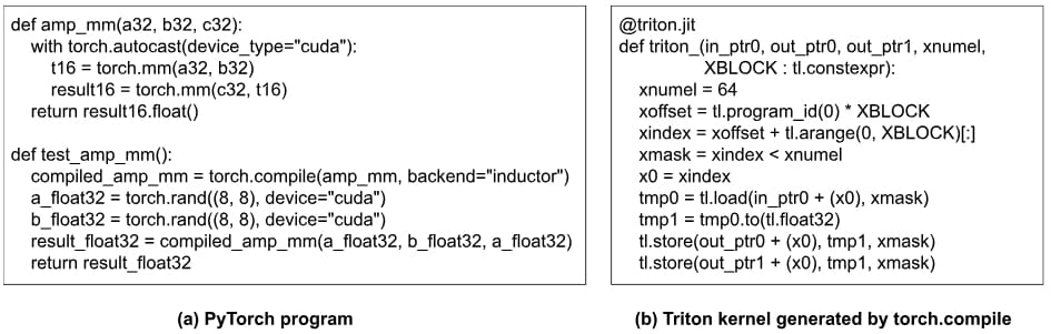
Fig. 2: How PT2 reduces type conversion overhead when using AMP.
- Reusing buffers on the GPU:
- With a global view, the scheduler in torch.compile can reuse buffers on the GPU, thereby reducing both memory allocation time and memory consumption. Figure 3 shows the driver program that calls the Triton kernels generated for the program in Figure 2(a). We can see that
buf1is reused asbuf4.
- With a global view, the scheduler in torch.compile can reuse buffers on the GPU, thereby reducing both memory allocation time and memory consumption. Figure 3 shows the driver program that calls the Triton kernels generated for the program in Figure 2(a). We can see that
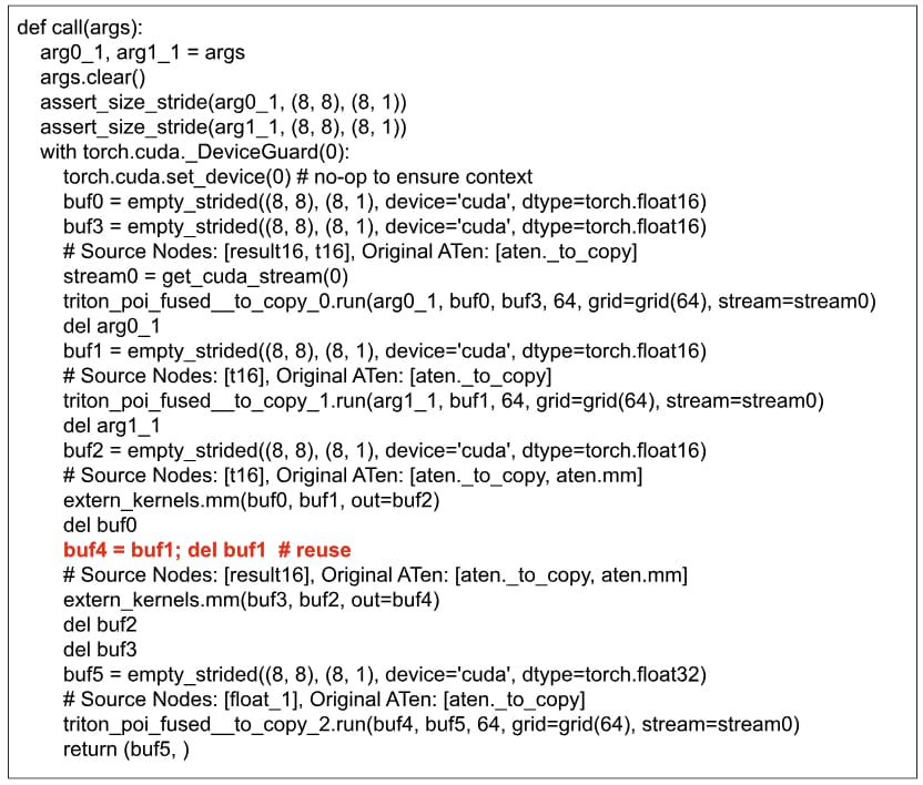
Fig. 3: Reuse of buffers.
- Autotuning:
- PT2 has options to enable autotuning (via Triton) on matrix-multiply ops, pointwise ops, and reduction ops. Tunable parameters include block size, number of stages, and number of warps. With autotuning, the most performant implementation of an op can be found empirically.
3. Production environment considerations
In this section, we describe a number of important considerations in applying PT2 to production.
3.1 Ensuring no model quality degradation with torch.compile
Applying torch.compile to a model will cause numerical changes because of (1) reordering of floating-point ops during various optimizations such as fusion and (2) use of lower precision data types like bf16 if AMP is enabled. Therefore 100% bitwise compatibility with PT 1.x is not expected. Nevertheless, we still need to make sure that the model quality (measured in some form of numeric scores) is preserved after applying torch.compile. Typically, each production model will have its own range of acceptable scores (e.g., percentage change must be within 0.01%).
In case of a model-quality drop caused by torch.compile, we need to do a deep-dive debug.
One useful technique for debugging a torch.compile-related numeric issue is to apply torch.compile with different backends, in particular “eager” and “aot_eager”, in addition to “inductor”:
- If the numeric issue happens with the “eager” backend, then the forward graph constructed by torch.compile is likely incorrect;
- If the numeric issue doesn’t happen with “eager” but happens with “aot_eager”, then the backward graph constructed by torch.compile is likely incorrect;
- If the numeric issue doesn’t happen with either “eager” or “aot_eager” but happens with “inductor”, then the code generation inside the inductor is likely incorrect.
3.2 Autotuning in production
By default, the autotuning in torch.inductor is done online _while the model is executed. For some production models, we find that the autotuning time can take several hours, which is not acceptable for production. Therefore, we add _offline autotuning which works as depicted in Figure 4. The very first time that a model is run, the details (e.g., input tensor shape, data type etc) on all ops that require tuning will be logged to a database. Then, a tuning process for these ops is run overnight to search for the most performant implementation of each op; the search result is updated to a persistent cache (implemented as a source file of torch.inductor). Next time when the model is run again, the tuned implementation of each op will be found in the cache and chosen for execution.
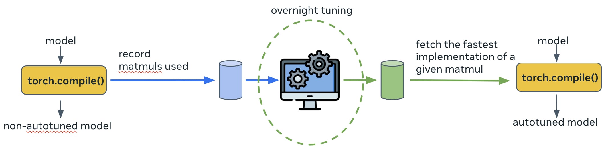
Fig. 4: The offline autotuning used in production.
As we previously discussed in this blog, a profiler is essential for debugging the performance of production models. We have enhanced the profiler to display torch.compile related events on the timeline. The most useful ones are marking which parts of the model are running compiled code so that we can quickly validate if the parts of the model that are supposed to be compiled are actually compiled by torch.compile. For example, the trace in Figure 5 has two compiled regions (with the label “CompiledFunction”). Other useful events are time spent on the compilation and that spent on accessing the compiler’s code-cache.
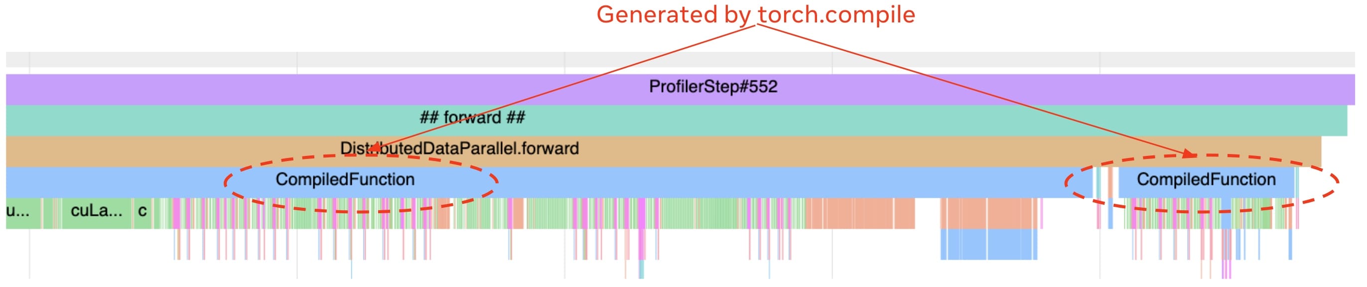
Fig. 5: A trace with two compiled regions.
3.4 Controlling just-in-time compilation time
torch.compile uses just-in-time compilation. The compilation happens when the first batch of data is trained. In our production setting, there is an upper limit on how much time is allowed for a training job to reach its first batch, aka Time-To-First-Batch (TTFB). We need to make sure that enabling torch.compile will not increase TTFB to over the limit. This could be challenging because production models are large and~~ ~~torch.compile can take substantial compilation time. We enable parallel compilation to keep the compile time under control (this is controlled by the global variable compile_threads inside torch/_inductor/config.py, which is already set to the CPU count on OSS Linux). A model is decomposed into one or more computational graphs; each graph is decomposed into multiple Triton kernels. If parallel compilation is enabled, all the Triton kernels in the same graph can be compiled simultaneously (nevertheless, kernels from different graphs are still compiled in serial). Figure 6 illustrates how parallel compilation helps.
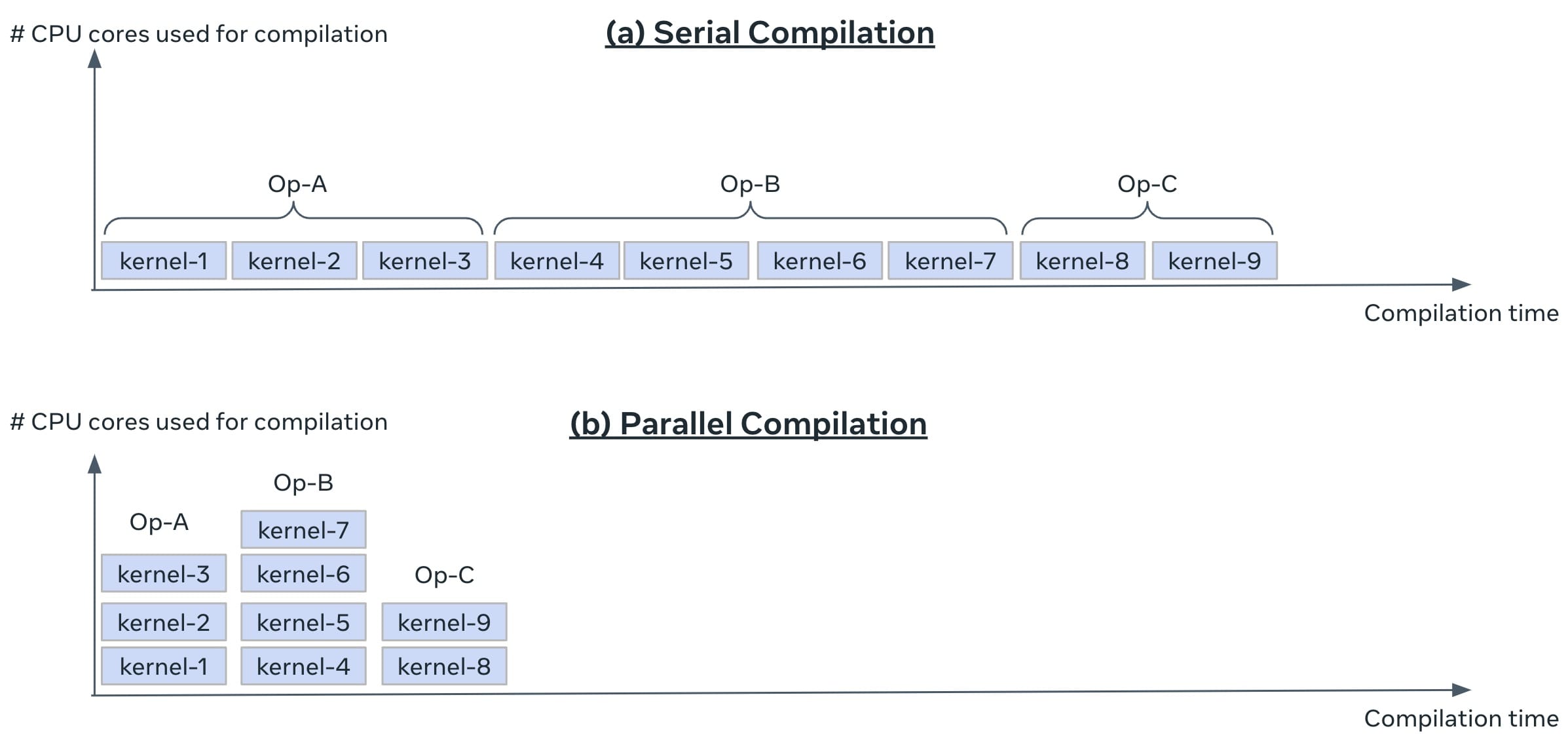
Fig. 6: Using parallel compilation in production.
4. Results
In this section, we use three production models to evaluate PT2. First we show the training time speedups with PT2, using different optimization configs. Second, we show the importance of parallel compilation on the compilation time.
4.1 Training-time speedup with torch.compile
Figure 7 reports the training-time speedup with PT2. For each model, we show four cases: (i) no-compile with bf16, (ii) compile with fp32, (iii) compile with bf16, (iv) compile with bf16 and autotuning. The y-axis is the speedup over the baseline, which is no-compile with fp32. Note that no-compile with bf16 is actually slower than no-compile with fp32, due to the type conversion overhead. In contrast, compiling with bf16 achieves much larger speedups by reducing much of this overhead. Overall, given that these models are already heavily optimized by hand, we are excited to see that torch.compile can still provide 1.14-1.24x speedup.
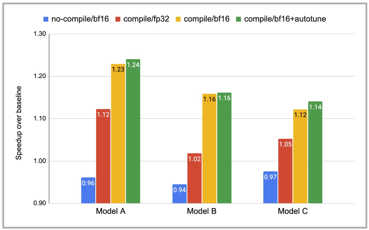
Fig. 7: Training-time speedup with torch.compile (note: the baseline, no-compile/fp32, is_ omitted _in this figure).
4.2 Compilation-time reduction with parallel compilation
Figure 8 shows the compilation time with and without parallel compilation. While there is still room for improvement on the serial compilation time, parallel compilation has reduced the compilation overhead on TTFB to an acceptable level. Models B and C benefit more from parallel compilation than Model A does because they have more distinct Triton kernels per graph.
Fig. 8: PT2 compilation time.
5. Concluding Remarks
In this blog, we demonstrate that PT2 can significantly accelerate the training of large and complex production AI models with reasonable compilation time. In our next blog, we will discuss how PT2 can do general graph transformations.
6. Acknowledgements
Many thanks to Mark Saroufim, Adnan Aziz, and Gregory Chanan for their detailed and insightful reviews.