Figure 1. Our implementation of recurrent model-free RL outperforms the on-policy version (PPO/A2C-GRU), and a recent model-based POMDP algorithm (VRM) on most tasks of a POMDP benchmark where VRM was evaluated in their paper.
While algorithms for decision-making typically focus on relatively easy problems where everything is known, most realistic problems involve noise and incomplete information. Complex algorithms have been proposed to tackle these complex problems, but there’s a simple approach that (in theory) works on both the easy and the complex problems. We show how to make this simple approach work in practice.
Why POMDPs?
Decision-making tasks in the real world are messy, with noise, occlusions, and uncertainty that are typically missing from their canonical problem formulation as a Markov decision process (MDP; Bellman, 1957). In contrast, Partially Observable MDPs (POMDPs; Åström, 1965) can capture the uncertainty in the states, rewards, and dynamics. Such uncertainty arises in applications such as robotics, healthcare, NLP and finance.
-
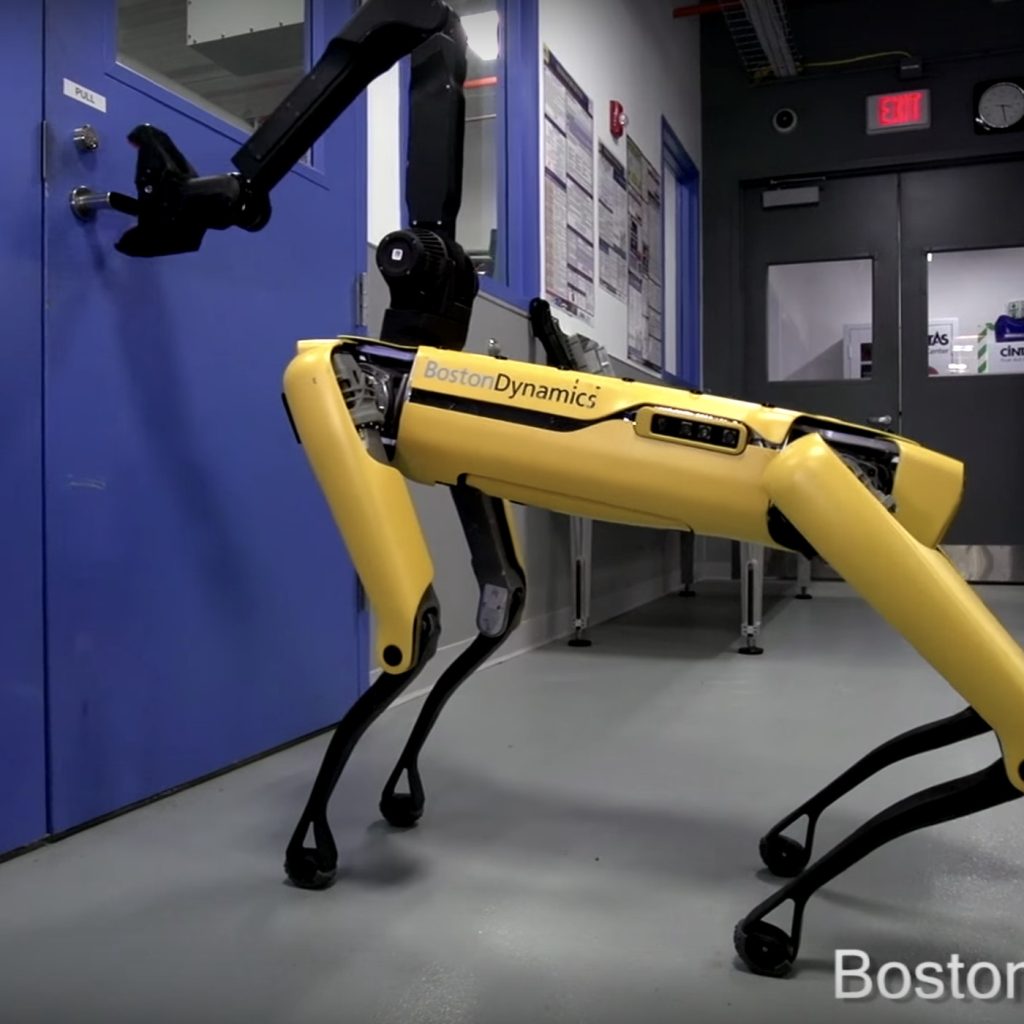
A robot has noisy sensors (from Boston Dynamics). -

A human has occlusion in the vision (René Magritte, The Son of Man, 1964).
Apart from being realistic, POMDPs are a general framework that contains many subareas in RL, including:
- Meta-RL (Schmidhuber, 1987, Thrun and Pratt, 2012, Duan et al., 2016, Wang et al., 2017): assume the hidden states (task variables) of a POMDP do not vary through time. For example, a robot has to discover which goal state it is supposed to reach.
- Robust RL (Bagnell et al., 2001, Rajeswaran et al., 2017, Pinto et al., 2017, Pattanaik et al., 2018): maximizing the worst-case returns over tasks. For example, the motor friction of a robot is unknown, and the goal is to learn a control policy that works for the worst-case choice of motor friction.
- Generalization in RL (Whiteson et al., 2011, Zhang et al., 2018, Packer et al., 2018, Cobbe et al., 2019): maximizing the returns over unseen tasks during testing.
- Temporal credit assignment (Sutton, 1984, Hung et al., 2018, Arjona-Medina et al., 2019, Ren et al., 2021): assume reward function is history-dependent.
What is recurrent model-free RL?
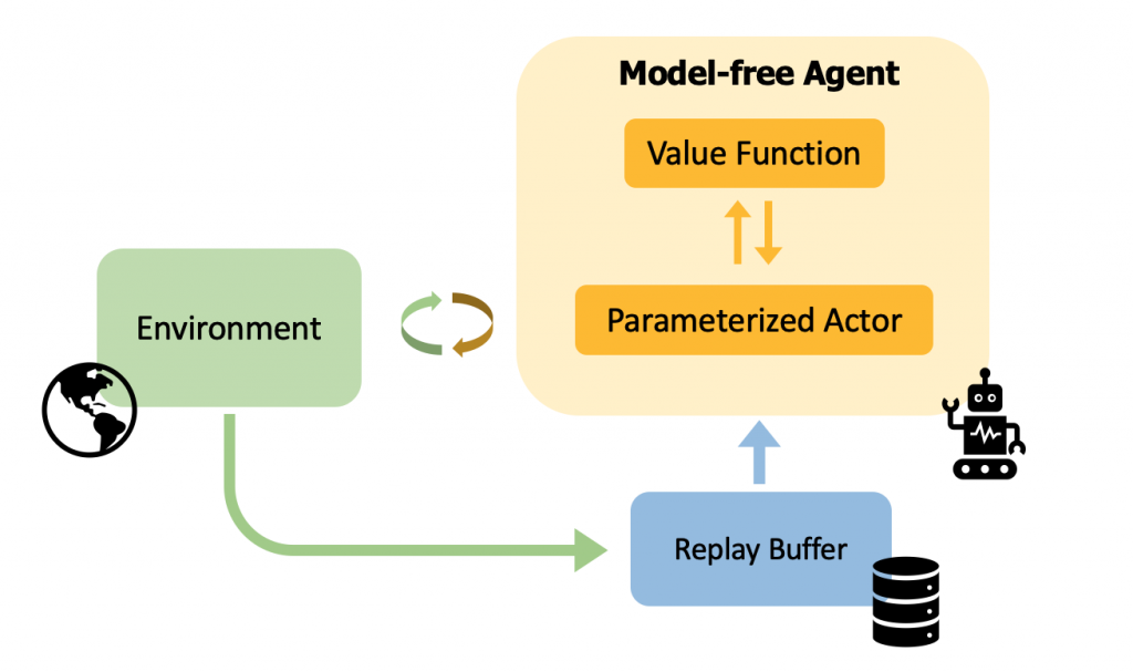
Solving POMDPs is hard because the agent needs to learn two tasks simultaneously: inference and control. Inference aims to infer the posterior over current states conditioned on history. Control aims to perform RL / planning algorithms on the inferred state space. While prior methods typically decouple the two jobs with separate models, deep learning, provides us with a general and simple baseline: combine an off-the-shelf RL algorithm with a recurrent neural network (RNN; e.g., LSTM (Hochreiter & Schmidhuber, 1997) and GRU (Chung et al., 2014)).
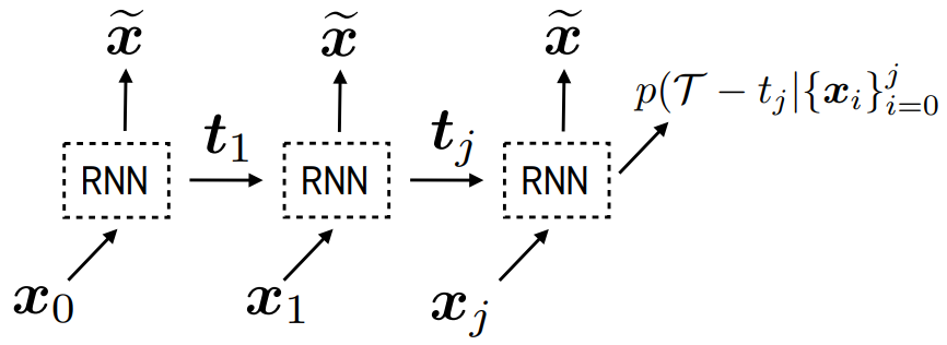
By backpropagating the gradients from policy loss, RNNs make it possible to process sequences (histories in POMDPs) and learn implicit inference on the state space for control. We refer to it as recurrent model-free RL. Fig. 2 presents our design, where actor and critic networks each have an RNN as the history encoder.

Recurrent model-free RL has many merits at first glance:
- Conceptually simple. The policy purely learns from rewards, without extra objectives.
- Easy to implement. Practitioners can just change several lines of code from model-free RL.
- Expressive in theory. RNNs have been shown as universal function approximators (Siegelmann & Sontag, 1995, Schäfer & Zimmermann, 2006) and, thus recurrent model-free RL can (approximately) express any memory-based policies.
Due to its simplicity and expressivity, there is rich literature (Schmidhuber, 1991, Bakker, 2001, Wierstra et al., 2007, Heess et al., 2015, Hausknecht & Stone, 2015) on studying different RL algorithms and RNN architectures of recurrent model-free RL. However, prior work has shown that it often fails in practice with poor or unstable performance (Igl et al., 2018, Hung et al., 2018, Packer et al., 2018, Rakelly et al., 2019, Zintgraf et al., 2020, Han et al., 2020, Zhang et al., 2021, Raposo et al., 2021), with only a few exceptions (Yu et al., 2019, Fakoor et al., 2020).
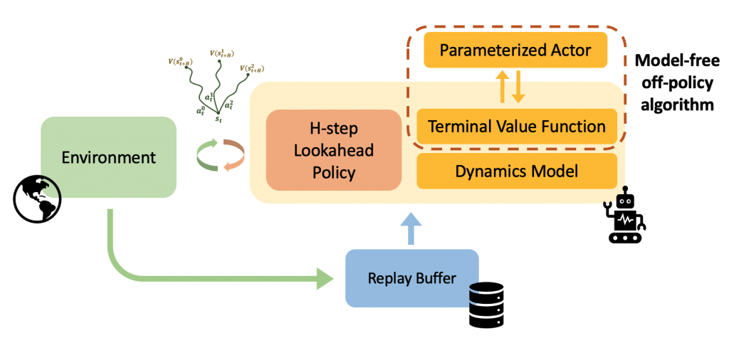
Motivated by the poor performance of this simple baseline, prior work has proposed more sophisticated methods. Some introduce model-based objectives that explicitly learn inference, while others incorporate the assumptions used in the subarea of POMDPs as inductive bias. Both achieve good results on a range of respective tasks, although the model-based methods may have staleness issue in the belief states stored in the replay buffer, and the specialized methods require more assumptions than recurrent model-free RL (e.g., meta-RL methods normally assumes the hidden variable is constant within a single episode).
How to train recurrent model-free RL?
In this work, we found that recurrent model-Free RL is not fatally failed, but just needed to be implemented differently, with differences including:
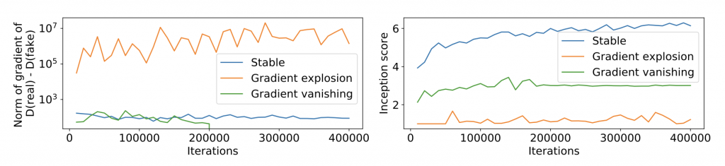
- Separating the RNNs in actor and critic networks. Un-sharing the weights can prevent gradient explosion, and can be the difference between the algorithm learning nothing and solving the task almost perfectly.
- Using an off-policy RL algorithm to improve sample efficiency. Using, say, TD3 instead of PPO greatly improves sample efficiency.
- Tuning the RNN context length. We found that the RNN architectures (LSTM and GRU) do not matter much, but the RNN context length (the length of the sequence fed into the RL algorithm), is crucial and depends on the task. We suggest choosing a medium length as a start.
Properly tuned, the simple baseline outperforms alternatives on many POMDPs
With these changes, our implementation of recurrent model-free RL is at least on par with (if not much better than) prior methods, on the tasks those prior methods were designed to solve. While prior methods are typically designed to solve special cases of POMDPs, recurrent model-free RL applies to all types of POMDPs.
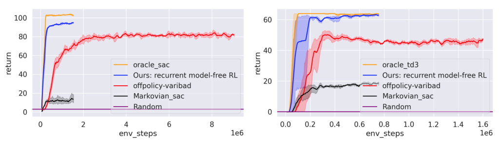
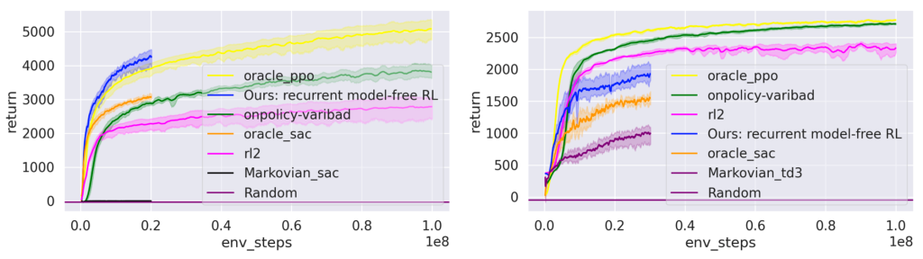
Our first comparison looks at meta-RL tasks, which are usually approached by methods that decouple the task inference and reward maximization steps (Rakelly et al., 2019, Zintgraf et al., 2020). When comparing these prototypical methods (on-policy variBAD (Zintgraf et al., 2020) and off-policy variBAD (Dorfman et al., 2020)), we find that our recurrent model-free approach can often perform at least on par with them. These results (Fig. 3, 4) suggest that disentangling inference and control may be not that necessary in many tasks.
Next, we move on to the robust RL setting, which is mostly solved by algorithms that explicitly maximize the worst returns (Rajeswaran et al., 2017, Mankowitz et al., 2020). By comparing one recent robust RL algorithm (Jiang et al., 2021), we find that our recurrent model-free approach performs better in all the tasks. The results (Fig. 5) indicate that with the power of implicit task inference with RNNs, we can improve both average and worst returns.

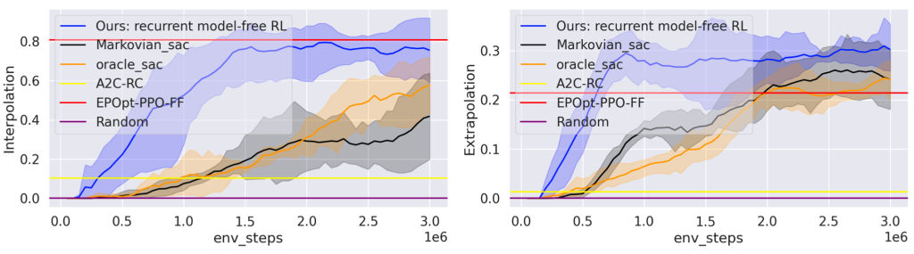
Then we explore the generalization in RL, where people have different kinds of specialized methods, including policy regularization (Farebrother et al., 2018) and data augmentation (Lee et al., 2020). Here we choose a popular benchmark SunBlaze (Packer et al., 2018) which provides a specialized baseline EPOpt-PPO-FF (Rajeswaran et al., 2017). The results (Fig. 6) show that despite not explicitly enhancing generalization, our recurrent model-free approach can perform better in extrapolation than the baseline. This suggests that the task inference learned by RNN is generalizable.
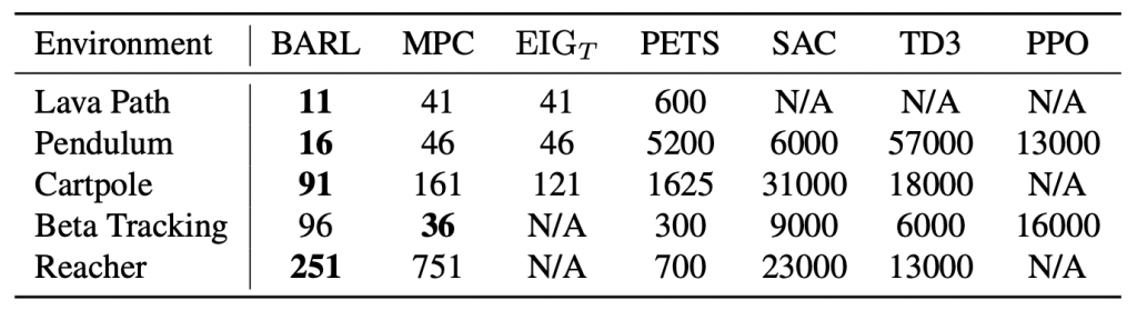
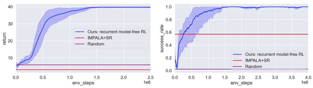
Finally, we study the temporal credit assignment domain where the methods for solving it usually involve reward decomposition/redistribution (Liu et al., 2019, Hung et al., 2018). Here, we choose a recent specialized method IMPALA+SR (Raposo et al., 2021), and evaluate our method on their benchmark with pixel-based discrete control and sparse rewards. Despite being unaware of the reward structure and not performing credit assignment explicitly, our recurrent model-free approach can perform better. The results (Fig. 7) indicate that recurrent policies can effectively cope with sparse rewards, perhaps better than previously expected.
Conclusion
In a sense, our finding can be interpreted as echoing the motivation for deep learning: we can achieve better results by reducing a method to a single differentiable architecture, optimized end-to-end with a single loss. This is exciting because RL systems often involve many interconnected parts (e.g., feature extracting, model learning, value estimation) trained with different objectives, but perhaps they might be replaced by end-to-end approaches if equipped with sufficiently expressive architectures.
We have open-sourced the code on GitHub to support reproducibility and to help future work develop better POMDP algorithms. Please see our project site for the paper and our ICML 2022 presentation.